SCALLOPS End-to-End Walkthrough: PERISCOPE Dataset Guide

Welcome to the primary hands-on tutorial for the SCALLOPS Command Line Interface. This notebook walks you through a complete, production-grade computational pipeline explicitly optimized for analyzing Optical Pooled Screens (OPS).

As detailed in the SCALLOPS bioRxiv preprint, SCALLOPS provides a highly scalable framework designed to handle the terabyte-scale image processing demands of pooled genetic screening. Unlike traditional workflows that decouple genetic data from morphology, OPS combines the scale of pooled libraries with high-content, image-based phenotypes. By leveraging in situ sequencing (ISS) of perturbation barcodes directly inside intact cells, SCALLOPS efficiently decodes and maps complex physical traits to precise genetic alterations at single-cell resolution.

Execution and Concurrency Note: To maintain clarity and provide a clean step-by-step narrative, this notebook executes SCALLOPS commands sequentially on a single machine. However, the SCALLOPS architecture is fundamentally built for massive, multi-node compute clusters. In production, nearly every stage of this pipeline can be scaled horizontally.

Interactive Tutorial Note: This workbook serves as an interactive guide using real, public data. To demonstrate the pipeline’s end-to-end execution, we will process a single plate from the Broad Institute PERISCOPE Dataset—a genome-wide CRISPR knockout screen in A549 cells.

Pipeline Architecture & Dependency Graph

When scaling from a local sandbox tutorial to a production-scale screen, understanding the exact data-dependency graph is vital. The SCALLOPS framework uses a production-grade execution graph (codified in its Workflow Description Language - WDL configurations) optimized for resource allocations.

The flowchart below outlines how data flows sequentially through bottlenecks and splits into highly concurrent parallel execution branches:

                  [Raw Image Input]
                         │
                         ▼
┌───────────────────────────────────────────────────────────┐
│ Module 1: Module-Specific Illumination Correction         │
└────────────────────────┬──────────────────────────────────┘
                         │ (Strict Flat-Field Dependency)
                         ▼
┌───────────────────────────────────────────────────────────┐
│ Module 2: Robust Graph-Based Image Stitching              │
└────────────────────────┬──────────────────────────────────┘
                         │ (Assembled OME Zarr Canvas)
                         ▼
       ┌─────────────────┴────────────────────────┐
       ▼ (Parallel Branch A: Sequencing)          ▼ (Parallel Branch B: Phenotype)
┌────────────────────────────────┐       ┌────────────────────────────────┐
│ Module 3: Sequencing (ISS)     │       │ Module 4: Cellular             │
│ Image Registration             │       │ Segmentation                   │
│ (Align cycles over time to t0) │       │ (Nuclei -> Cell boundaries)    │
└──────────────┬─────────────────┘       └──────────────┬─────────────────┘
               │                                        │
               ▼                                        ▼
┌────────────────────────────────┐       ┌────────────────────────────────┐
│ Module 5: Spot Detection       │       │ Module 6: Subcellular Objects  │
│ (Cycle-wise standard dev.)     │       │ & Morphology Feature Engine    │
└──────────────┬─────────────────┘       └──────────────┬─────────────────┘
               │                                        │
               └─────────────────┬──────────────────────┘
                                 │ (Branch Synchronization Merge)
                                 ▼
                  ┌──────────────────────────────┐
                  │ Module 7: Base Calling &     │
                  │ White-List Barcode Decoding  │
                  └──────────────┬───────────────┘
                                 │
                                 ▼
                  ┌──────────────────────────────┐
                  │ Module 8: Downstream Merging │
                  │ & Registration QC Analysis   │
                  └──────────────────────────────┘

The Parallelization & Dependency Rules:

The Serialization Bottleneck (Modules 1 ➔ 2): Stitching has an unyielding dependency on illumination correction (when required; some instruments already correct for this). The tile engine requires the generated flatfield profile to dynamically normalize pixel intensities when writing out the unified OME Zarr arrays.
The Concurrent Core Split (Modules 3 ║ 4): Once your raw data is assembled into standardized OME Zarr formats, the pipeline splits into two highly independent pathways that can run simultaneously across multiple machines:
- Branch A (Sequencing Operations): Runs multi-cycle registration over time to track micro-shifts in the microscope stage across days of fluidic chemistry. Once aligned, it immediately launches spot detection.
- Branch B (Phenotypic Segmentation & Extraction): Segments cellular and nuclear masks out-of-core. As soon as the labels are written, the engine fires off highly parallel feature extraction tasks to capture thousands of morphometric, intensity, and texture metrics per cell compartment.
The Synchronization Checkpoint (Module 7): The branches merge back together at the Base Calling stage. The read decoding engine takes the transcript spot locations computed in Branch A and overlays them directly onto the cell boundaries isolated in Branch B to cleanly call guide RNA barcodes at a single-cell level.
Consolidation (Module 8): The pipeline concludes by merging the structural metrics, decoded tracking barcodes, and alignment quality tables into a clean, analysis-ready dataframe.

Step 1: Environment Setup and Tool Configuration

Before processing our microscopy data, we need to prepare our terminal environment and install the necessary dependencies.

Notebook Kernel Requirement: Because this tutorial interacts entirely with a live terminal workflow via system binaries, your Jupyter Notebook kernel must be set to Bash. If you do not have a native Bash kernel available in your environment, you can quickly add it using Python by executing pip install bash_kernel and running python -m bash_kernel.install in your base terminal before reopening this sheet.

For this tutorial, we will use uv, an extremely fast Python package installer and resolver written in Rust. However, you are welcome to recreate these steps using standard pip or any environment manager of your choice.

If you do not have uv installed on your machine yet, you can quickly install it via curl (on macOS/Linux):

[ ]:

curl -LsSf https://astral.sh/uv/install.sh | sh

Or using Homebrew/Chocolatey depending on your operating system. Once uv is ready, we will create a dedicated virtual environment, activate it, and install the scallops package directly through our terminal.

Create a new virtual environment using uv

uv venv scallops_env

Activate the virtual environment

On macOS/Linux:

source scallops_env/bin/activate # On Windows (Command Prompt): # scallops_env:nbsphinx-math:Scripts\activate.bat

Install scallops directly into our isolated environment

uv pip install scallops

Verify that the scallops CLI tool is correctly installed and accessible

scallops –help

We will define our primary environment variables at the parent images/ directory. This allows the SCALLOPS engine to dynamically map out the plate and well structures from the file tree while using our subset anchor to lock focus onto the target plate.

[1]:

# Define the core screen batch name and the target plate
export BATCH="20200805_A549_WG_Screen"
export PLATE="CP186A"
export WELL="1"

# Set the public S3 image directory root and your local runtime workspace
export INPUT_BUCKET="s3://cellpainting-gallery/cpg0021-periscope/broad/images/${BATCH}/images/"
export OUTPUT_DIR="scallops_run/${PLATE}"

# set anonymous for public s3
export FSSPEC_S3_ANON=True
export AWS_SHARED_CREDENTIALS_FILE=/dev/null

# Verify configurations
echo "Processing Screen Batch: ${BATCH}"
echo "Target Plate ID: ${PLATE}"
echo "Target Well ID ${WELL}"
echo "Source S3 Repository URI: ${INPUT_BUCKET}"
echo "Local Execution Workspace: ${OUTPUT_DIR}"

Processing Screen Batch: 20200805_A549_WG_Screen
Target Plate ID: CP186A
Target Well ID 1
Source S3 Repository URI: s3://cellpainting-gallery/cpg0021-periscope/broad/images/20200805_A549_WG_Screen/images/
Local Execution Workspace: scallops_run/CP186A

We will now run the illumination correction aggregation routine to eliminate systemic optical vignetting across the plate. This calculation is computed independently for each well, cycle, and channel by calculating the mean (or median) across tiles, applying a median filter with a disk footprint radius of 1/20th of the image area, and rescaling using the 2nd percentile for a robust minimum. This method is equivalent to running CellProfiler’s CorrectIlluminationCalculate module with “Regular”, “All”, and “Median Filter” settings.

Because the Barcoding (SBS) cycles and Phenotypic Profiling (Cell Painting) rounds utilize completely different optical paths and exposures, we run these correction steps as two separate commands.

To handle variations between uppercase 10X and lowercase 10x folder names across the 12 sequencing rounds, we use a flexible prefix wildcard ({skip}_c{t}-SBS-{skip}) to extract the cycle index (t). We append --subset "${PLATE}-${WELL}*" to ensure the engine only processes one well belonging to our active plate, as an example in this tutorial.

[2]:

scallops illum-corr agg \
  --agg-method mean \
  --images "$INPUT_BUCKET" \
  --image-pattern "{plate}/{skip}_c{t}-SBS-{skip}/Well{well}_Point{skip}_{skip}_Channel{skip}_Seq{skip}.nd2" \
  --output "${OUTPUT_DIR}/stitch/iss/illumination_correction/" \
  --groupby plate well t \
  --subset "${PLATE}-${WELL}-*" \
  --force

06/02/2026 15:11 - Scallops version: 1.0.0
06/02/2026 15:11 - Scallops command:
scallops illum-corr agg --agg-method mean --images s3://cellpainting-gallery/cpg0021-periscope/broad/images/20200805_A549_WG_Screen/images/ --image-pattern {plate}/{skip}_c{t}-SBS-{skip}/Well{well}_Point{skip}_{skip}_Channel{skip}_Seq{skip}.nd2 --output scallops_run/CP186A//stitch/iss/illumination_correction/ --groupby plate well t --subset CP186A-1-*
06/02/2026 15:12 - Running illumination correction for CP186A-1-12.
06/02/2026 15:12 - 320 tiles.
06/02/2026 15:12 - Running illumination correction for CP186A-1-6.
06/02/2026 15:12 - 320 tiles.
06/02/2026 15:12 - Running illumination correction for CP186A-1-9.
06/02/2026 15:12 - Running illumination correction for CP186A-1-3.
06/02/2026 15:12 - 320 tiles.
06/02/2026 15:12 - Running illumination correction for CP186A-1-10.
06/02/2026 15:12 - 320 tiles.
06/02/2026 15:12 - Running illumination correction for CP186A-1-4.
06/02/2026 15:12 - 320 tiles.
06/02/2026 15:12 - Running illumination correction for CP186A-1-7.
06/02/2026 15:12 - 320 tiles.
06/02/2026 15:12 - Running illumination correction for CP186A-1-1.
06/02/2026 15:12 - 320 tiles.
06/02/2026 15:12 - 320 tiles.
06/02/2026 15:12 - Running illumination correction for CP186A-1-8.
06/02/2026 15:12 - Running illumination correction for CP186A-1-11.
06/02/2026 15:12 - 320 tiles.
06/02/2026 15:12 - 320 tiles.
06/02/2026 15:12 - Running illumination correction for CP186A-1-5.
06/02/2026 15:12 - Running illumination correction for CP186A-1-2.
06/02/2026 15:12 - 320 tiles.
06/02/2026 15:12 - 320 tiles.
06/02/2026 15:22 - Smooth: 186
06/02/2026 15:22 - Smooth: 186
06/02/2026 15:22 - Smooth: 186
06/02/2026 15:22 - Smooth: 186
06/02/2026 15:22 - Smooth: 186
06/02/2026 15:22 - Smooth: 186
06/02/2026 15:22 - Smooth: 186
06/02/2026 15:22 - Smooth: 186
06/02/2026 15:22 - Smooth: 186
06/02/2026 15:22 - Smooth: 186
06/02/2026 15:22 - Smooth: 186
06/02/2026 15:22 - Smooth: 186
06/02/2026 15:23 - Processing done in 00H:12M:25S

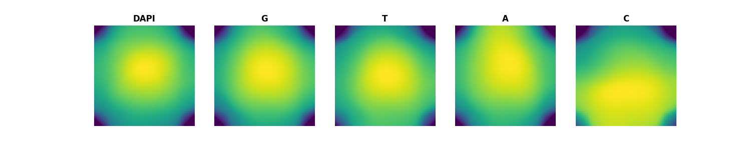
This will generate one 5D (t, c, z, y, x) tiff file per each well and cycle, and will be passed to the sticher later on:

[3]:

ls ${OUTPUT_DIR}/stitch/iss/illumination_correction | head

CP186A-1-1.ome.tiff
CP186A-1-10.ome.tiff
CP186A-1-11.ome.tiff
CP186A-1-12.ome.tiff
CP186A-1-2.ome.tiff
CP186A-1-3.ome.tiff
CP186A-1-4.ome.tiff
CP186A-1-5.ome.tiff
CP186A-1-6.ome.tiff
CP186A-1-7.ome.tiff

[4]:

python3 << 'EOF' | display
import matplotlib
matplotlib.use('Agg')
import sys
from scallops.io import read_image
import matplotlib.pyplot as plt
from pathlib import Path
img = read_image('scallops_run/CP186A/stitch/iss/illumination_correction/CP186A-1-1.ome.tiff')
f, axes = plt.subplots(ncols=5, figsize=(15, 3))
for ax, (i, ch) in zip(axes, enumerate(['DAPI', 'G', 'T', 'A', 'C'])):
    ax.imshow(img.isel(t=0, c=i, z=0))
    ax.axis('off')
    ax.set_title(ch)
f.savefig(sys.stdout.buffer, format='png')
plt.close()
EOF

The image ends with .ome.tiff, which might indicate an OME-TIFF file format. You might want to install the `bioio-ome-tiff` plug-in for improved metadata Processing.You can also use 'bioio.plugin_feasibility_report(image)' method to check if a specific image can be handled by the available plugins.

../_images/notebooks_End-to-End_10_1.png

For the phenotype channels, the files reside globally under a single folder layout (20X_CP_CP186A/). Because there is no shifting time, cycle dimension or multiple phenotipic rounds (t) inside this run, we drop t from our tracking and group the calculation strictly by plate and well. However if you have multiple rounds of phenotyping (e.g. FISH, IF1, IF2, etc) you can set t as said rounds. Note that 1 and 2 can be started concurrently in separate machines. In fact we could make it concurrent to the well level (which our WDL does).

[6]:

scallops illum-corr agg \
  --agg-method mean \
  --images "$INPUT_BUCKET" \
  --image-pattern "{plate}/20X_CP_{plate}/Well{well}_Point{skip}_{skip}_Channel{skip}_Seq{skip}.nd2" \
  --output "${OUTPUT_DIR}/stitch/pheno/illumination_correction/" \
  --groupby plate well \
  --subset "${PLATE}-${WELL}" \
  --force

06/02/2026 15:35 - Scallops version: 1.0.0
06/02/2026 15:35 - Scallops command:
scallops illum-corr agg --agg-method mean --images s3://cellpainting-gallery/cpg0021-periscope/broad/images/20200805_A549_WG_Screen/images/ --image-pattern {plate}/20X_CP_{plate}/Well{well}_Point{skip}_{skip}_Channel{skip}_Seq{skip}.nd2 --output scallops_run/CP186A//stitch/pheno/illumination_correction/ --groupby plate well --subset CP186A-1
06/02/2026 15:36 - Running illumination correction for CP186A-1.
06/02/2026 15:36 - 1,364 tiles.
06/02/2026 15:40 - Smooth: 186
06/02/2026 15:41 - Processing done in 00H:05M:42S

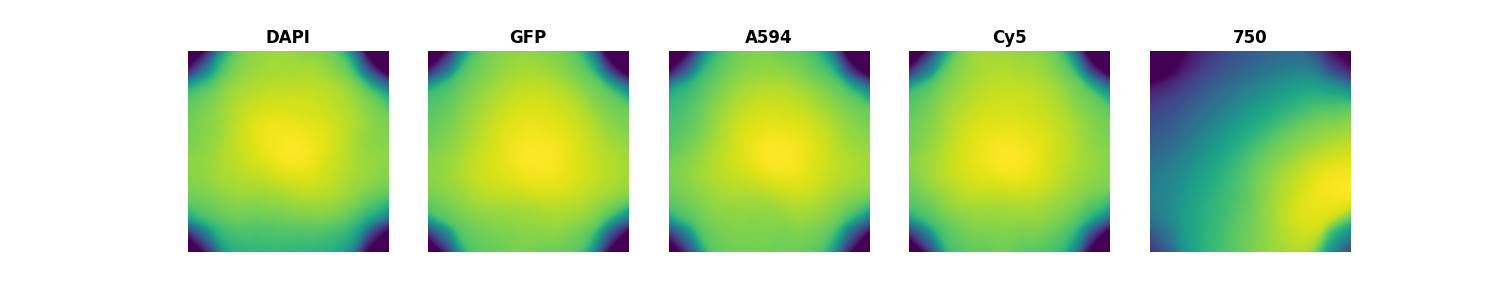
For the phenotype, you would only get one tiff per well pwe round:

[7]:

ls ${OUTPUT_DIR}/stitch/pheno/illumination_correction

CP186A-1.ome.tiff

[8]:

python3 << 'EOF'| display
import matplotlib
matplotlib.use('Agg')
import sys
from scallops.io import read_image
import matplotlib.pyplot as plt
from pathlib import Path
img = read_image('scallops_run/CP186A/stitch/pheno/illumination_correction/CP186A-1.ome.tiff')
f, axes = plt.subplots(ncols=5, figsize=(15, 3))
for ax, (i, ch) in zip(axes, enumerate(['DAPI', 'GFP', 'A594', 'Cy5', '750'])):
    ax.imshow(img.isel(t=0, c=i, z=0))
    ax.axis('off')
    ax.set_title(ch)
f.savefig(sys.stdout.buffer, format='png')
plt.close()
EOF

The image ends with .ome.tiff, which might indicate an OME-TIFF file format. You might want to install the `bioio-ome-tiff` plug-in for improved metadata Processing.You can also use 'bioio.plugin_feasibility_report(image)' method to check if a specific image can be handled by the available plugins.

../_images/notebooks_End-to-End_15_1.png

With our flat-field illumination profiles generated, the next step is to assemble individual high-magnification image tiles into a continuous mosaic.

SCALLOPS stitches each well and cycle independently into standard, highly interoperable OME Zarr multi-scale images. The microscope stage positions are parsed natively from raw instrument formats (including .nd2). As the engine writes the stitched output image, it actively divides raw pixel intensities by our computed flat-field images to apply the illumination correction on the fly.

Metadata Tracking Tip: In the updated commands below, we have explicitly mapped {tile} and {ChannelInfo} variables within our filename pattern matchers. By capturing {ChannelInfo} as a discrete wildcard instead of skipping it, SCALLOPS will automatically retain and inject this vital channel configuration directly into your stitched OME Zarr image metadata array rather than dropping it.

Just like the pre-processing step, we will run the stitching process separately for the Sequencing (SBS) data and the Phenotypic Profiling (Cell Painting) data.

We point the --ffp (flat-field profile) argument to our freshly generated SBS illumination correction directory. We use the wildcard combination ${PLATE}-* to ensure all wells and sequencing cycles are stitched.

[9]:

scallops stitch \
  --images "$INPUT_BUCKET" \
  --image-pattern "{plate}/{skip}_c{t}-SBS-{skip}/Well{well}_Point{skip}_{tile}_Channel{ChannelInfo}_Seq{skip}.nd2" \
  --ffp "${OUTPUT_DIR}/stitch/iss/illumination_correction/{plate}-{well}-{t}.ome.tiff" \
  --image-output "${OUTPUT_DIR}/stitch/iss/stitch/stitch.zarr" \
  --report-output "${OUTPUT_DIR}/stitch/iss/stitch/report" \
  --groupby plate well t \
  --subset "${PLATE}-${WELL}-*"

06/02/2026 15:41 - Scallops version: 1.0.0
06/02/2026 15:41 - Scallops command:
scallops stitch --images s3://cellpainting-gallery/cpg0021-periscope/broad/images/20200805_A549_WG_Screen/images/ --image-pattern {plate}/{skip}_c{t}-SBS-{skip}/Well{well}_Point{skip}_{tile}_Channel{ChannelInfo}_Seq{skip}.nd2 --ffp scallops_run/CP186A//stitch/iss/illumination_correction/{plate}-{well}-{t}.ome.tiff --image-output scallops_run/CP186A//stitch/iss/stitch/stitch.zarr --report-output scallops_run/CP186A//stitch/iss/stitch/report --groupby plate well t --subset CP186A-1-*
06/02/2026 15:43 - Running stitching for CP186A-1-10.
06/02/2026 15:43 - 320 tiles.
06/02/2026 15:43 - Running stitching for CP186A-1-4.
06/02/2026 15:43 - 320 tiles.
06/02/2026 15:44 - Flip y axis: false, flip x axis: true, swap axes: false, and minimum tile overlap: 0.03.
06/02/2026 15:44 - Found 599 edges.
06/02/2026 15:44 - Computing radial correction K.
06/02/2026 15:44 - Flip y axis: false, flip x axis: true, swap axes: false, and minimum tile overlap: 0.03.
06/02/2026 15:44 - Found 599 edges.
06/02/2026 15:44 - Computing radial correction K.
06/02/2026 15:44 - Radial correction K: 1e-08, crop width: 4.
06/02/2026 15:44 - Computing null distribution.
[##                                      ] | 5% Completed | 10.32 s06/02/2026 15:44 - Radial correction K: 1e-08, crop width: 4.
06/02/2026 15:44 - Computing null distribution.
[########################################] | 100% Completed | 39.51 s
06/02/2026 15:45 - Null distribution median: 0.1578, standard deviation estimated from MAD: 0.0560.
06/02/2026 15:45 - Computing tile shifts.
[########################################] | 100% Completed | 35.27 s
06/02/2026 15:45 - Null distribution median: 0.1491, standard deviation estimated from MAD: 0.0560.
06/02/2026 15:45 - Computing tile shifts.
[########################################] | 100% Completed | 36.04 s
06/02/2026 15:45 - Optimizing tile positions.
06/02/2026 15:45 - Kept 599 / 599 edges after filtering using null distribution.
06/02/2026 15:45 - Kept 599 / 599 edges after filtering using max shift.
06/02/2026 15:45 - Edges in spanning tree: 319 / 599.
[############################            ] | 71% Completed | 29.32 s06/02/2026 15:45 - Crop for writing: 48.
06/02/2026 15:45 - Evaluating stitching quality using 1,183 overlaps.
[########################################] | 100% Completed | 33.07 s
06/02/2026 15:46 - Optimizing tile positions.
06/02/2026 15:46 - Kept 599 / 599 edges after filtering using null distribution.
06/02/2026 15:46 - Kept 599 / 599 edges after filtering using max shift.
06/02/2026 15:46 - Edges in spanning tree: 319 / 599.
[                                        ] | 0% Completed | 3.17 s06/02/2026 15:46 - Crop for writing: 48.
06/02/2026 15:46 - Evaluating stitching quality using 1,183 overlaps.
[########################################] | 100% Completed | 32.70 s
06/02/2026 15:46 - ZNCC: 0.9248.
06/02/2026 15:46 - Saving report to scallops_run/CP186A//stitch/iss/stitch/report/CP186A-1-4.pdf.
[########################################] | 100% Completed | 30.11 s
06/02/2026 15:46 - ZNCC: 0.9288.
06/02/2026 15:46 - Saving report to scallops_run/CP186A//stitch/iss/stitch/report/CP186A-1-10.pdf.
06/02/2026 15:46 - Fusing channels 0, 1, 2, 3, 4.
[                                        ] | 0% Completed | 655.00 ms06/02/2026 15:46 - Fusing channels 0, 1, 2, 3, 4.
[########################################] | 100% Completed | 39.71 s
06/02/2026 15:47 - Writing to disk.
[########################################] | 100% Completed | 42.84 s
06/02/2026 15:47 - Writing to disk.
[########################################] | 100% Completed | 5.67 ss
[                                        ] | 0% Completed | 4.02 s06/02/2026 15:47 - Running stitching for CP186A-1-9.
06/02/2026 15:47 - 320 tiles.
[########################################] | 100% Completed | 6.29 s
06/02/2026 15:47 - Running stitching for CP186A-1-3.
06/02/2026 15:47 - 320 tiles.
06/02/2026 15:48 - Flip y axis: false, flip x axis: true, swap axes: false, and minimum tile overlap: 0.03.
06/02/2026 15:48 - Found 599 edges.
06/02/2026 15:48 - Computing radial correction K.
06/02/2026 15:48 - Radial correction K: 1e-08, crop width: 4.
06/02/2026 15:48 - Computing null distribution.
[##################################      ] | 87% Completed | 35.66 s06/02/2026 15:49 - Flip y axis: false, flip x axis: true, swap axes: false, and minimum tile overlap: 0.03.
06/02/2026 15:49 - Found 599 edges.
06/02/2026 15:49 - Computing radial correction K.
[########################################] | 100% Completed | 37.42 s
06/02/2026 15:49 - Null distribution median: 0.1554, standard deviation estimated from MAD: 0.0563.
06/02/2026 15:49 - Computing tile shifts.
[###########                             ] | 29% Completed | 19.62 s06/02/2026 15:49 - Radial correction K: 1e-08, crop width: 4.
06/02/2026 15:49 - Computing null distribution.
[########################################] | 100% Completed | 36.69 s
06/02/2026 15:50 - Optimizing tile positions.
06/02/2026 15:50 - Kept 599 / 599 edges after filtering using null distribution.
06/02/2026 15:50 - Kept 599 / 599 edges after filtering using max shift.
06/02/2026 15:50 - Edges in spanning tree: 319 / 599.
[#########                               ] | 22% Completed | 16.66 s06/02/2026 15:50 - Crop for writing: 48.
06/02/2026 15:50 - Evaluating stitching quality using 1,183 overlaps.
[########################################] | 100% Completed | 34.89 s
06/02/2026 15:50 - Null distribution median: 0.1478, standard deviation estimated from MAD: 0.0528.
06/02/2026 15:50 - Computing tile shifts.
[########################################] | 100% Completed | 31.80 s
06/02/2026 15:50 - ZNCC: 0.9258.
06/02/2026 15:50 - Saving report to scallops_run/CP186A//stitch/iss/stitch/report/CP186A-1-3.pdf.
[###########                             ] | 29% Completed | 17.44 s06/02/2026 15:50 - Fusing channels 0, 1, 2, 3, 4.
[########################################] | 100% Completed | 33.48 s
06/02/2026 15:50 - Optimizing tile positions.
06/02/2026 15:50 - Kept 599 / 599 edges after filtering using null distribution.
06/02/2026 15:50 - Kept 599 / 599 edges after filtering using max shift.
06/02/2026 15:50 - Edges in spanning tree: 319 / 599.
[#######                                 ] | 19% Completed | 15.89 s06/02/2026 15:50 - Crop for writing: 48.
06/02/2026 15:50 - Evaluating stitching quality using 1,183 overlaps.
[########################################] | 100% Completed | 40.66 s
06/02/2026 15:51 - Writing to disk.
[########################################] | 100% Completed | 30.17 s
06/02/2026 15:51 - ZNCC: 0.9283.
[                                        ] | 0% Completed | 2.04 s06/02/2026 15:51 - Saving report to scallops_run/CP186A//stitch/iss/stitch/report/CP186A-1-9.pdf.
[#######################                 ] | 57% Completed | 5.48 s06/02/2026 15:51 - Fusing channels 0, 1, 2, 3, 4.
[########################################] | 100% Completed | 5.93 ss
[                                        ] | 0% Completed | 1.22 s06/02/2026 15:51 - Running stitching for CP186A-1-12.
06/02/2026 15:51 - 320 tiles.
[########################################] | 100% Completed | 38.65 s
06/02/2026 15:52 - Writing to disk.
[                                        ] | 0% Completed | 703.46 ms06/02/2026 15:52 - Flip y axis: false, flip x axis: true, swap axes: false, and minimum tile overlap: 0.03.
06/02/2026 15:52 - Found 599 edges.
06/02/2026 15:52 - Computing radial correction K.
[########################################] | 100% Completed | 6.20 ss
06/02/2026 15:52 - Running stitching for CP186A-1-8.
06/02/2026 15:52 - 320 tiles.
06/02/2026 15:52 - Radial correction K: 1e-08, crop width: 4.
06/02/2026 15:52 - Computing null distribution.
[##########################              ] | 66% Completed | 31.98 s06/02/2026 15:53 - Flip y axis: false, flip x axis: true, swap axes: false, and minimum tile overlap: 0.03.
06/02/2026 15:53 - Found 599 edges.
06/02/2026 15:53 - Computing radial correction K.
[########################################] | 100% Completed | 37.33 s
06/02/2026 15:53 - Null distribution median: 0.1458, standard deviation estimated from MAD: 0.0524.
06/02/2026 15:53 - Computing tile shifts.
[#########                               ] | 23% Completed | 16.90 s06/02/2026 15:53 - Radial correction K: 1e-08, crop width: 4.
06/02/2026 15:53 - Computing null distribution.
[########################################] | 100% Completed | 36.42 s
06/02/2026 15:53 - Optimizing tile positions.
06/02/2026 15:53 - Kept 599 / 599 edges after filtering using null distribution.
06/02/2026 15:53 - Kept 599 / 599 edges after filtering using max shift.
06/02/2026 15:53 - Edges in spanning tree: 319 / 599.
[##########                              ] | 26% Completed | 19.04 s06/02/2026 15:53 - Crop for writing: 48.
06/02/2026 15:53 - Evaluating stitching quality using 1,183 overlaps.
[########################################] | 100% Completed | 35.85 s
06/02/2026 15:54 - Null distribution median: 0.1488, standard deviation estimated from MAD: 0.0528.
06/02/2026 15:54 - Computing tile shifts.
[########################################] | 100% Completed | 31.18 s
06/02/2026 15:54 - ZNCC: 0.9293.
06/02/2026 15:54 - Saving report to scallops_run/CP186A//stitch/iss/stitch/report/CP186A-1-12.pdf.
[#############                           ] | 33% Completed | 18.35 s06/02/2026 15:54 - Fusing channels 0, 1, 2, 3, 4.
[########################################] | 100% Completed | 33.13 s
06/02/2026 15:54 - Optimizing tile positions.
06/02/2026 15:54 - Kept 599 / 599 edges after filtering using null distribution.
06/02/2026 15:54 - Kept 599 / 599 edges after filtering using max shift.
06/02/2026 15:54 - Edges in spanning tree: 319 / 599.
[#######                                 ] | 19% Completed | 14.74 s06/02/2026 15:54 - Crop for writing: 48.
06/02/2026 15:54 - Evaluating stitching quality using 1,183 overlaps.
[########################################] | 100% Completed | 39.45 s
06/02/2026 15:55 - Writing to disk.
[########################################] | 100% Completed | 30.03 s
06/02/2026 15:55 - ZNCC: 0.9199.
06/02/2026 15:55 - Saving report to scallops_run/CP186A//stitch/iss/stitch/report/CP186A-1-8.pdf.
[########                                ] | 20% Completed | 5.30 s06/02/2026 15:55 - Fusing channels 0, 1, 2, 3, 4.
[########################################] | 100% Completed | 6.03 ss
[                                        ] | 0% Completed | 1.45 s06/02/2026 15:55 - Running stitching for CP186A-1-11.
06/02/2026 15:55 - 320 tiles.
[########################################] | 100% Completed | 39.25 s
06/02/2026 15:55 - Writing to disk.
[########################################] | 100% Completed | 5.29 ss
06/02/2026 15:56 - Running stitching for CP186A-1-7.
06/02/2026 15:56 - 320 tiles.
06/02/2026 15:56 - Flip y axis: false, flip x axis: true, swap axes: false, and minimum tile overlap: 0.03.
06/02/2026 15:56 - Found 599 edges.
06/02/2026 15:56 - Computing radial correction K.
06/02/2026 15:56 - Flip y axis: false, flip x axis: true, swap axes: false, and minimum tile overlap: 0.03.
06/02/2026 15:56 - Found 599 edges.
06/02/2026 15:56 - Computing radial correction K.
06/02/2026 15:57 - Radial correction K: 1e-08, crop width: 4.
06/02/2026 15:57 - Computing null distribution.
[                                        ] | 0% Completed | 2.27 s06/02/2026 15:57 - Radial correction K: 1e-08, crop width: 4.
06/02/2026 15:57 - Computing null distribution.
[########################################] | 100% Completed | 35.69 s
06/02/2026 15:57 - Null distribution median: 0.1448, standard deviation estimated from MAD: 0.0531.
06/02/2026 15:57 - Computing tile shifts.
[########################################] | 100% Completed | 36.21 s
06/02/2026 15:57 - Null distribution median: 0.1441, standard deviation estimated from MAD: 0.0527.
06/02/2026 15:57 - Computing tile shifts.
[########################################] | 100% Completed | 33.12 s
06/02/2026 15:58 - Optimizing tile positions.
06/02/2026 15:58 - Kept 599 / 599 edges after filtering using null distribution.
06/02/2026 15:58 - Kept 599 / 599 edges after filtering using max shift.
06/02/2026 15:58 - Edges in spanning tree: 319 / 599.
[############################            ] | 71% Completed | 29.95 s06/02/2026 15:58 - Crop for writing: 48.
06/02/2026 15:58 - Evaluating stitching quality using 1,183 overlaps.
[########################################] | 100% Completed | 34.21 s
06/02/2026 15:58 - Optimizing tile positions.
06/02/2026 15:58 - Kept 599 / 599 edges after filtering using null distribution.
06/02/2026 15:58 - Kept 599 / 599 edges after filtering using max shift.
06/02/2026 15:58 - Edges in spanning tree: 319 / 599.
[                                        ] | 0% Completed | 3.61 s06/02/2026 15:58 - Crop for writing: 48.
06/02/2026 15:58 - Evaluating stitching quality using 1,183 overlaps.
[########################################] | 100% Completed | 30.31 s
06/02/2026 15:58 - ZNCC: 0.9297.
06/02/2026 15:58 - Saving report to scallops_run/CP186A//stitch/iss/stitch/report/CP186A-1-7.pdf.
[###############################         ] | 79% Completed | 29.50 s06/02/2026 15:58 - Fusing channels 0, 1, 2, 3, 4.
[########################################] | 100% Completed | 31.81 s
06/02/2026 15:58 - ZNCC: 0.9298.
06/02/2026 15:58 - Saving report to scallops_run/CP186A//stitch/iss/stitch/report/CP186A-1-11.pdf.
[                                        ] | 1% Completed | 5.63 s06/02/2026 15:58 - Fusing channels 0, 1, 2, 3, 4.
[########################################] | 100% Completed | 38.41 s
06/02/2026 15:59 - Writing to disk.
[########################################] | 100% Completed | 39.79 s
06/02/2026 15:59 - Writing to disk.
[########################################] | 100% Completed | 5.47 s
06/02/2026 15:59 - Running stitching for CP186A-1-6.
06/02/2026 15:59 - 320 tiles.
[########################################] | 100% Completed | 6.09 ss
06/02/2026 15:59 - Running stitching for CP186A-1-2.
06/02/2026 15:59 - 320 tiles.
06/02/2026 16:00 - Flip y axis: false, flip x axis: true, swap axes: false, and minimum tile overlap: 0.03.
06/02/2026 16:00 - Found 599 edges.
06/02/2026 16:00 - Computing radial correction K.
06/02/2026 16:00 - Flip y axis: false, flip x axis: true, swap axes: false, and minimum tile overlap: 0.03.
06/02/2026 16:00 - Found 599 edges.
06/02/2026 16:00 - Computing radial correction K.
06/02/2026 16:00 - Radial correction K: 1e-08, crop width: 4.
06/02/2026 16:00 - Computing null distribution.
[##                                      ] | 5% Completed | 11.12 s06/02/2026 16:00 - Radial correction K: 7.900000000000001e-09, crop width: 3.
06/02/2026 16:00 - Computing null distribution.
[########################################] | 100% Completed | 35.96 s
06/02/2026 16:01 - Null distribution median: 0.1447, standard deviation estimated from MAD: 0.0532.
06/02/2026 16:01 - Computing tile shifts.
[########################################] | 100% Completed | 35.93 s
06/02/2026 16:01 - Null distribution median: 0.1587, standard deviation estimated from MAD: 0.0584.
06/02/2026 16:01 - Computing tile shifts.
[########################################] | 100% Completed | 33.34 s
06/02/2026 16:01 - Optimizing tile positions.
06/02/2026 16:01 - Kept 599 / 599 edges after filtering using null distribution.
06/02/2026 16:01 - Kept 599 / 599 edges after filtering using max shift.
06/02/2026 16:01 - Edges in spanning tree: 319 / 599.
[#################                       ] | 44% Completed | 21.78 s06/02/2026 16:01 - Crop for writing: 48.
06/02/2026 16:01 - Evaluating stitching quality using 1,183 overlaps.
[########################################] | 100% Completed | 34.15 s
06/02/2026 16:02 - Optimizing tile positions.
06/02/2026 16:02 - Kept 599 / 599 edges after filtering using null distribution.
06/02/2026 16:02 - Kept 599 / 599 edges after filtering using max shift.
06/02/2026 16:02 - Edges in spanning tree: 319 / 599.
[####                                    ] | 10% Completed | 11.88 s06/02/2026 16:02 - Crop for writing: 48.
06/02/2026 16:02 - Evaluating stitching quality using 1,183 overlaps.
[########################################] | 100% Completed | 30.01 s
06/02/2026 16:02 - ZNCC: 0.9280.
06/02/2026 16:02 - Saving report to scallops_run/CP186A//stitch/iss/stitch/report/CP186A-1-6.pdf.
[################                        ] | 42% Completed | 20.95 s06/02/2026 16:02 - Fusing channels 0, 1, 2, 3, 4.
[########################################] | 100% Completed | 31.03 s
06/02/2026 16:02 - ZNCC: 0.9238.
06/02/2026 16:02 - Saving report to scallops_run/CP186A//stitch/iss/stitch/report/CP186A-1-2.pdf.
[######                                  ] | 17% Completed | 13.56 s06/02/2026 16:02 - Fusing channels 0, 1, 2, 3, 4.
[########################################] | 100% Completed | 38.69 s
06/02/2026 16:03 - Writing to disk.
[########################################] | 100% Completed | 5.54 ss
[############################            ] | 70% Completed | 35.29 s06/02/2026 16:03 - Running stitching for CP186A-1-5.
06/02/2026 16:03 - 320 tiles.
[########################################] | 100% Completed | 40.22 s
06/02/2026 16:03 - Writing to disk.
[########################################] | 100% Completed | 5.44 ss
06/02/2026 16:03 - Running stitching for CP186A-1-1.
06/02/2026 16:03 - 320 tiles.
06/02/2026 16:04 - Flip y axis: false, flip x axis: true, swap axes: false, and minimum tile overlap: 0.03.
06/02/2026 16:04 - Found 599 edges.
06/02/2026 16:04 - Computing radial correction K.
06/02/2026 16:04 - Flip y axis: false, flip x axis: true, swap axes: false, and minimum tile overlap: 0.03.
06/02/2026 16:04 - Found 599 edges.
06/02/2026 16:04 - Computing radial correction K.
06/02/2026 16:04 - Radial correction K: 1e-08, crop width: 4.
06/02/2026 16:04 - Computing null distribution.
[                                        ] | 0% Completed | 2.33 s06/02/2026 16:04 - Radial correction K: 1e-08, crop width: 4.
06/02/2026 16:04 - Computing null distribution.
[########################################] | 100% Completed | 35.62 s
06/02/2026 16:05 - Null distribution median: 0.1546, standard deviation estimated from MAD: 0.0562.
06/02/2026 16:05 - Computing tile shifts.
[########################################] | 100% Completed | 35.35 s
06/02/2026 16:05 - Null distribution median: 0.1701, standard deviation estimated from MAD: 0.0552.
06/02/2026 16:05 - Computing tile shifts.
[########################################] | 100% Completed | 32.34 s
06/02/2026 16:05 - Optimizing tile positions.
06/02/2026 16:05 - Kept 599 / 599 edges after filtering using null distribution.
06/02/2026 16:05 - Kept 599 / 599 edges after filtering using max shift.
06/02/2026 16:05 - Edges in spanning tree: 319 / 599.
[##########################              ] | 67% Completed | 29.85 s06/02/2026 16:05 - Crop for writing: 48.
06/02/2026 16:05 - Evaluating stitching quality using 1,183 overlaps.
[########################################] | 100% Completed | 33.74 s
06/02/2026 16:05 - Optimizing tile positions.
06/02/2026 16:05 - Kept 599 / 599 edges after filtering using null distribution.
06/02/2026 16:05 - Kept 599 / 599 edges after filtering using max shift.
06/02/2026 16:05 - Edges in spanning tree: 319 / 599.
06/02/2026 16:05 - Crop for writing: 48.
06/02/2026 16:05 - Evaluating stitching quality using 1,183 overlaps.
[########################################] | 100% Completed | 30.22 s
[########################                ] | 62% Completed | 26.25 s06/02/2026 16:06 - ZNCC: 0.9284.
06/02/2026 16:06 - Saving report to scallops_run/CP186A//stitch/iss/stitch/report/CP186A-1-5.pdf.
[##################################      ] | 87% Completed | 29.73 s06/02/2026 16:06 - Fusing channels 0, 1, 2, 3, 4.
[########################################] | 100% Completed | 30.67 s
[                                        ] | 0% Completed | 785.02 ms06/02/2026 16:06 - ZNCC: 0.9182.
06/02/2026 16:06 - Saving report to scallops_run/CP186A//stitch/iss/stitch/report/CP186A-1-1.pdf.
[                                        ] | 0% Completed | 4.35 s06/02/2026 16:06 - Fusing channels 0, 1, 2, 3, 4.
[########################################] | 100% Completed | 38.40 s
06/02/2026 16:06 - Writing to disk.
[########################################] | 100% Completed | 39.32 s
06/02/2026 16:06 - Writing to disk.
[########################################] | 100% Completed | 5.20 s
[########################################] | 100% Completed | 5.06 ss
06/02/2026 16:07 - Processing done in 00H:25M:12S

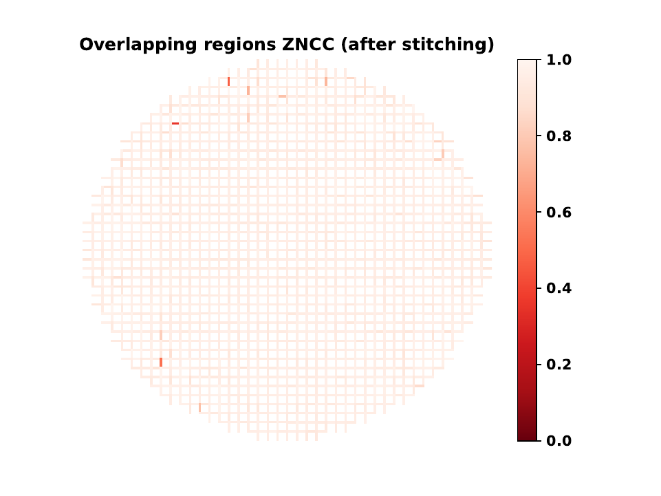
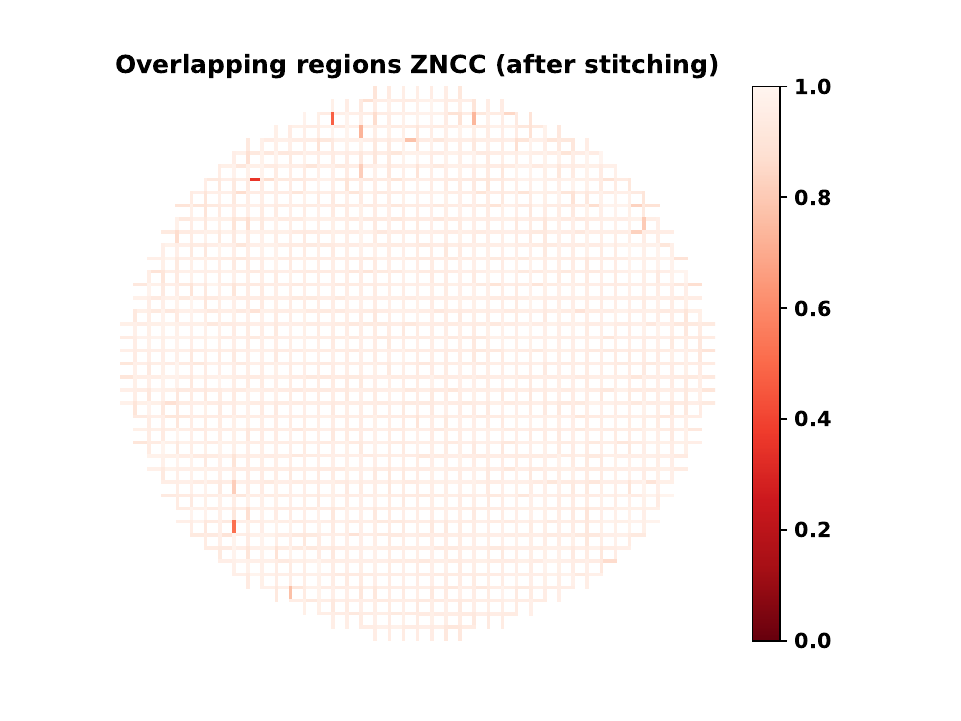
SCALLOPS produces a report (in whatever path you passed in --report-output), which contains parquet files with the positions of the tiles (*-positions.parquet), and the zncc score evaluation of the overlaps (*-eval.parquet). It will also contain a PDF with some QC reports, among which is the visualization of the overlapping regions zncc:

[1]:

pdftoppm -png -f 2 -l 2 -r 150 scallops_run/CP186A/stitch/iss/stitch/report/CP186A-1-1.pdf | display -jpeg

../_images/notebooks_End-to-End_19_0.png

For the phenotype data, we run a parallel stitching process pointing to the phenotype illumination correction directory. Since there is no shifting time dimension (t) inside the folder structure, our --ffp path reflects the simpler {plate}-{well}.ome.tiff schema, and the dataset is grouped cleanly by plate and well.

[4]:

scallops stitch \
  --images "$INPUT_BUCKET" \
  --image-pattern "{plate}/20X_CP_{plate}/Well{well}_Point{skip}_{tile}_Channel{ChannelInfo}_Seq{skip}.nd2" \
  --ffp "${OUTPUT_DIR}/stitch/pheno/illumination_correction/{plate}-{well}.ome.tiff" \
  --image-output "${OUTPUT_DIR}/stitch/pheno/stitch/stitch.zarr" \
  --report-output "${OUTPUT_DIR}/stitch/pheno/stitch/report" \
  --groupby plate well \
  --subset "${PLATE}-${WELL}"

06/02/2026 17:26 - Scallops version: 1.0.0
06/02/2026 17:26 - Scallops command:
scallops stitch --images s3://cellpainting-gallery/cpg0021-periscope/broad/images/20200805_A549_WG_Screen/images/ --image-pattern {plate}/20X_CP_{plate}/Well{well}_Point{skip}_{tile}_Channel{ChannelInfo}_Seq{skip}.nd2 --ffp scallops_run/CP186A//stitch/pheno/illumination_correction/{plate}-{well}.ome.tiff --image-output scallops_run/CP186A//stitch/pheno/stitch/stitch.zarr --report-output scallops_run/CP186A//stitch/pheno/stitch/report --groupby plate well --subset CP186A-1
06/02/2026 17:27 - Running stitching for CP186A-1.
06/02/2026 17:27 - 1,364 tiles.
06/02/2026 17:30 - Flip y axis: false, flip x axis: true, swap axes: false, and minimum tile overlap: 0.03.
06/02/2026 17:30 - Found 2,644 edges.
06/02/2026 17:30 - Computing radial correction K.
06/02/2026 17:30 - Radial correction K: 1e-08, crop width: 4.
06/02/2026 17:30 - Computing null distribution.
[########################################] | 100% Completed | 107.60 s
06/02/2026 17:32 - Null distribution median: 0.1840, standard deviation estimated from MAD: 0.0695.
06/02/2026 17:32 - Computing tile shifts.
[########################################] | 100% Completed | 158.01 s
06/02/2026 17:35 - Optimizing tile positions.
06/02/2026 17:35 - Kept 2,644 / 2,644 edges after filtering using null distribution.
06/02/2026 17:35 - Kept 2,643 / 2,644 edges after filtering using max shift.
06/02/2026 17:35 - Edges in spanning tree: 1,363 / 2,643.
06/02/2026 17:35 - Crop for writing: 53.
06/02/2026 17:35 - Evaluating stitching quality using 5,254 overlaps.
[########################################] | 100% Completed | 142.15 s
06/02/2026 17:37 - ZNCC: 0.9423.
06/02/2026 17:37 - Saving report to scallops_run/CP186A//stitch/pheno/stitch/report/CP186A-1.pdf.
06/02/2026 17:38 - Fusing channels 0, 1, 2, 3, 4.
[########################################] | 100% Completed | 184.57 s
06/02/2026 17:41 - Writing to disk.
[########################################] | 100% Completed | 24.97 s
06/02/2026 17:41 - Processing done in 00H:15M:23S

[1]:

pdftoppm -png -f 2 -l 2 -r 150 scallops_run/CP186A/stitch/pheno/stitch/report/CP186A-1.pdf | display -jpeg

../_images/notebooks_End-to-End_22_0.png

Now that all sequencing rounds and phenotypic images are fully stitched, we must align them into a single coherent spatial workspace.

In an Optical Pooled Screen, the barcode sequence inside each cell is read out sequentially over multiple successive rounds of sequencing-by-synthesis (SBS) chemistry. Over days of fluidic cycles, minor micro-shifts in the microscope stage can occur. To accurately trace individual transcript spots across all rounds, every sequential ISS cycle must be registered back to a baseline coordinate system—typically the very first imaging cycle.

SCALLOPS executes this process efficiently using the elastix registration engine. It computes the necessary spatial transformation matrices and saves the aligned outputs into an optimized, multi-cycle OME Zarr array.

PERISCOPE Workflow Note: In workflows with multiple disparate phenotypic imaging rounds (such as separate FISH and Immunofluorescence cycles), you would typically run an intermediate intra-phenotype registration step to align them. Because our target PERISCOPE dataset features a single, unified 20X Cell Painting round alongside our 10X sequencing cycles, we skip intra-phenotype alignment and can pass our stitched phenotype data straight into the cellular segmentation phase downstream!

Run the following command to register your 12 sequencing cycles:

[3]:

scallops registration elastix \
  --groupby plate well \
  --moving-image-pattern '{plate}-{well}-{t}' \
  --moving "${OUTPUT_DIR}/stitch/iss/stitch/stitch.zarr/" \
  --moving-output "${OUTPUT_DIR}/ops/iss-registered-t0.zarr" \
  --transform-output "${OUTPUT_DIR}/ops/iss-transforms-t0" \
  --subset "${PLATE}-${WELL}"

06/02/2026 17:45 - Scallops version: 1.0.0
06/02/2026 17:45 - Scallops command:
scallops registration elastix --groupby plate well --moving-image-pattern {plate}-{well}-{t} --moving scallops_run/CP186A//stitch/iss/stitch/stitch.zarr/ --moving-output scallops_run/CP186A//ops/iss-registered-t0.zarr --transform-output scallops_run/CP186A//ops/iss-transforms-t0 --subset CP186A-1
06/02/2026 17:46 - Running registration for CP186A-1 t=0
06/02/2026 17:46 - 12 inputs: CP186A-1-1, CP186A-1-2, CP186A-1-3, CP186A-1-4, CP186A-1-5, CP186A-1-6, CP186A-1-7, CP186A-1-8, CP186A-1-9, CP186A-1-10, CP186A-1-11, CP186A-1-12
06/02/2026 17:46 - Writing t=0, c=0.
06/02/2026 17:46 - Writing t=0, c=1.
06/02/2026 17:46 - Writing t=0, c=2.
06/02/2026 17:46 - Writing t=0, c=3.
06/02/2026 17:46 - Writing t=0, c=4.
06/02/2026 17:46 - Registering t=1 to t=0.
06/02/2026 17:46 - Center of mass shift microns: 15.4, 42.5
06/02/2026 17:46 - Initialized registration using 776 landmarks. Transformation: 1.00, 0.00, -0.00, 1.00, -16.10, 5.84.
06/02/2026 17:47 - Writing t=1, c=0.
06/02/2026 17:47 - Writing t=1, c=1.
06/02/2026 17:47 - Writing t=1, c=2.
06/02/2026 17:47 - Writing t=1, c=3.
06/02/2026 17:47 - Writing t=1, c=4.
06/02/2026 17:47 - Registering t=2 to t=0.
06/02/2026 17:48 - Center of mass shift microns: -1.3, 1.8
06/02/2026 17:48 - Initialized registration using 445 landmarks. Transformation: 1.00, -0.00, 0.00, 1.00, 1.38, -1.64.
06/02/2026 17:49 - Writing t=2, c=0.
06/02/2026 17:49 - Writing t=2, c=1.
06/02/2026 17:49 - Writing t=2, c=2.
06/02/2026 17:49 - Writing t=2, c=3.
06/02/2026 17:49 - Writing t=2, c=4.
06/02/2026 17:49 - Registering t=3 to t=0.
06/02/2026 17:49 - Center of mass shift microns: -46.1, -20.7
06/02/2026 17:50 - Initialized registration using 568 landmarks. Transformation: 1.00, -0.00, 0.00, 1.00, -2.57, 1.97.
06/02/2026 17:50 - Writing t=3, c=0.
06/02/2026 17:50 - Writing t=3, c=1.
06/02/2026 17:50 - Writing t=3, c=2.
06/02/2026 17:51 - Writing t=3, c=3.
06/02/2026 17:51 - Writing t=3, c=4.
06/02/2026 17:51 - Registering t=4 to t=0.
06/02/2026 17:51 - Center of mass shift microns: 3.7, 67.9
06/02/2026 17:51 - Initialized registration using 484 landmarks. Transformation: 1.00, -0.00, 0.00, 1.00, 0.05, -0.30.
06/02/2026 17:52 - Writing t=4, c=0.
06/02/2026 17:52 - Writing t=4, c=1.
06/02/2026 17:52 - Writing t=4, c=2.
06/02/2026 17:52 - Writing t=4, c=3.
06/02/2026 17:52 - Writing t=4, c=4.
06/02/2026 17:52 - Registering t=5 to t=0.
06/02/2026 17:53 - Center of mass shift microns: -32.4, 16.2
06/02/2026 17:53 - Initialized registration using 370 landmarks. Transformation: 1.00, -0.00, -0.00, 1.00, -3.17, 2.15.
06/02/2026 17:54 - Writing t=5, c=0.
06/02/2026 17:54 - Writing t=5, c=1.
06/02/2026 17:54 - Writing t=5, c=2.
06/02/2026 17:54 - Writing t=5, c=3.
06/02/2026 17:54 - Writing t=5, c=4.
06/02/2026 17:54 - Registering t=6 to t=0.
06/02/2026 17:54 - Center of mass shift microns: 106.5, 2.1
06/02/2026 17:55 - Initialized registration using 284 landmarks. Transformation: 1.00, -0.00, -0.00, 1.00, -1.11, 1.57.
06/02/2026 17:55 - Writing t=6, c=0.
06/02/2026 17:55 - Writing t=6, c=1.
06/02/2026 17:55 - Writing t=6, c=2.
06/02/2026 17:56 - Writing t=6, c=3.
06/02/2026 17:56 - Writing t=6, c=4.
06/02/2026 17:56 - Registering t=7 to t=0.
06/02/2026 17:56 - Center of mass shift microns: 21.8, 33.0
06/02/2026 17:56 - Initialized registration using 323 landmarks. Transformation: 1.00, -0.00, 0.00, 1.00, 2.11, -1.51.
06/02/2026 17:57 - Writing t=7, c=0.
06/02/2026 17:57 - Writing t=7, c=1.
06/02/2026 17:57 - Writing t=7, c=2.
06/02/2026 17:57 - Writing t=7, c=3.
06/02/2026 17:57 - Writing t=7, c=4.
06/02/2026 17:57 - Registering t=8 to t=0.
06/02/2026 17:58 - Center of mass shift microns: 13.0, 35.3
06/02/2026 17:58 - Initialized registration using 466 landmarks. Transformation: 1.00, -0.00, -0.00, 1.00, -0.95, 2.22.
06/02/2026 17:59 - Writing t=8, c=0.
06/02/2026 17:59 - Writing t=8, c=1.
06/02/2026 17:59 - Writing t=8, c=2.
06/02/2026 17:59 - Writing t=8, c=3.
06/02/2026 17:59 - Writing t=8, c=4.
06/02/2026 17:59 - Registering t=9 to t=0.
06/02/2026 17:59 - Center of mass shift microns: 13.5, 96.4
06/02/2026 18:00 - Initialized registration using 344 landmarks. Transformation: 1.00, 0.00, -0.00, 1.00, -5.36, 1.63.
06/02/2026 18:00 - Writing t=9, c=0.
06/02/2026 18:00 - Writing t=9, c=1.
06/02/2026 18:00 - Writing t=9, c=2.
06/02/2026 18:00 - Writing t=9, c=3.
06/02/2026 18:00 - Writing t=9, c=4.
06/02/2026 18:01 - Registering t=10 to t=0.
06/02/2026 18:01 - Center of mass shift microns: 117.8, 11.5
06/02/2026 18:01 - Initialized registration using 462 landmarks. Transformation: 1.00, -0.00, -0.00, 1.00, -4.14, -0.87.
06/02/2026 18:02 - Writing t=10, c=0.
06/02/2026 18:02 - Writing t=10, c=1.
06/02/2026 18:02 - Writing t=10, c=2.
06/02/2026 18:02 - Writing t=10, c=3.
06/02/2026 18:02 - Writing t=10, c=4.
06/02/2026 18:02 - Registering t=11 to t=0.
06/02/2026 18:02 - Center of mass shift microns: 62.3, 86.4
06/02/2026 18:03 - Initialized registration using 415 landmarks. Transformation: 1.00, 0.00, -0.00, 1.00, 0.28, 2.22.
06/02/2026 18:03 - Writing t=11, c=0.
06/02/2026 18:04 - Writing t=11, c=1.
06/02/2026 18:04 - Writing t=11, c=2.
06/02/2026 18:04 - Writing t=11, c=3.
06/02/2026 18:04 - Writing t=11, c=4.
06/02/2026 18:04 - Processing done in 00H:19M:02S

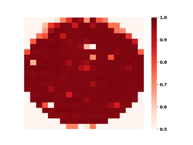
One useful proxy for goodness of registration is visualizing the minimum correlation between cells of every cycle to T0. Below an approximation using chunks of the image:

[4]:

python3 << 'EOF' | display

import matplotlib
matplotlib.use('Agg')
import matplotlib.pyplot as plt

import sys
import numpy as np
import dask.array as da
import seaborn as sns
from scallops.io import read_experiment

# read the registration using SCALLOPS' read_experiment
image = (
    read_experiment(
        "scallops_run/CP186A/ops/iss-registered-t0.zarr", dask=True
    )
        .images["CP186A-1"]
        .isel(c=0) # Select only dapi channel
    .squeeze()
)

# Set a function to apply to chunks to compute the minimum correlation
# between all cycles and the first as proxy for goodness of registration
def min_corr(a):
    corr_matrix = np.corrcoef(a.reshape(a.shape[0], -1))
    np.fill_diagonal(corr_matrix, 1.0)
    min_val = corr_matrix.min()
    if np.isnan(min_val):
        min_val = 0.0
    return np.full((1,) * 2, min_val)

min_corr_matrix = (
    da.map_blocks(min_corr, image.data, dtype=float, drop_axis=0).compute().squeeze()
)

fig, ax = plt.subplots()
sns.heatmap(min_corr_matrix, vmin=0.5, vmax=1, cmap="Reds", ax=ax)
ax.axis("off")
fig.savefig(sys.stdout.buffer, format='png')
plt.close()
EOF

/home/ubuntu/.venv/lib/python3.11/site-packages/numpy/lib/_function_base_impl.py:3023: RuntimeWarning: invalid value encountered in divide
  c /= stddev[:, None]
/home/ubuntu/.venv/lib/python3.11/site-packages/numpy/lib/_function_base_impl.py:3024: RuntimeWarning: invalid value encountered in divide
  c /= stddev[None, :]

../_images/notebooks_End-to-End_26_1.png

With our multi-scale OME Zarr arrays successfully stitched, we transition into the phenotypic profiling arm of our core pipeline: Cellular Segmentation.

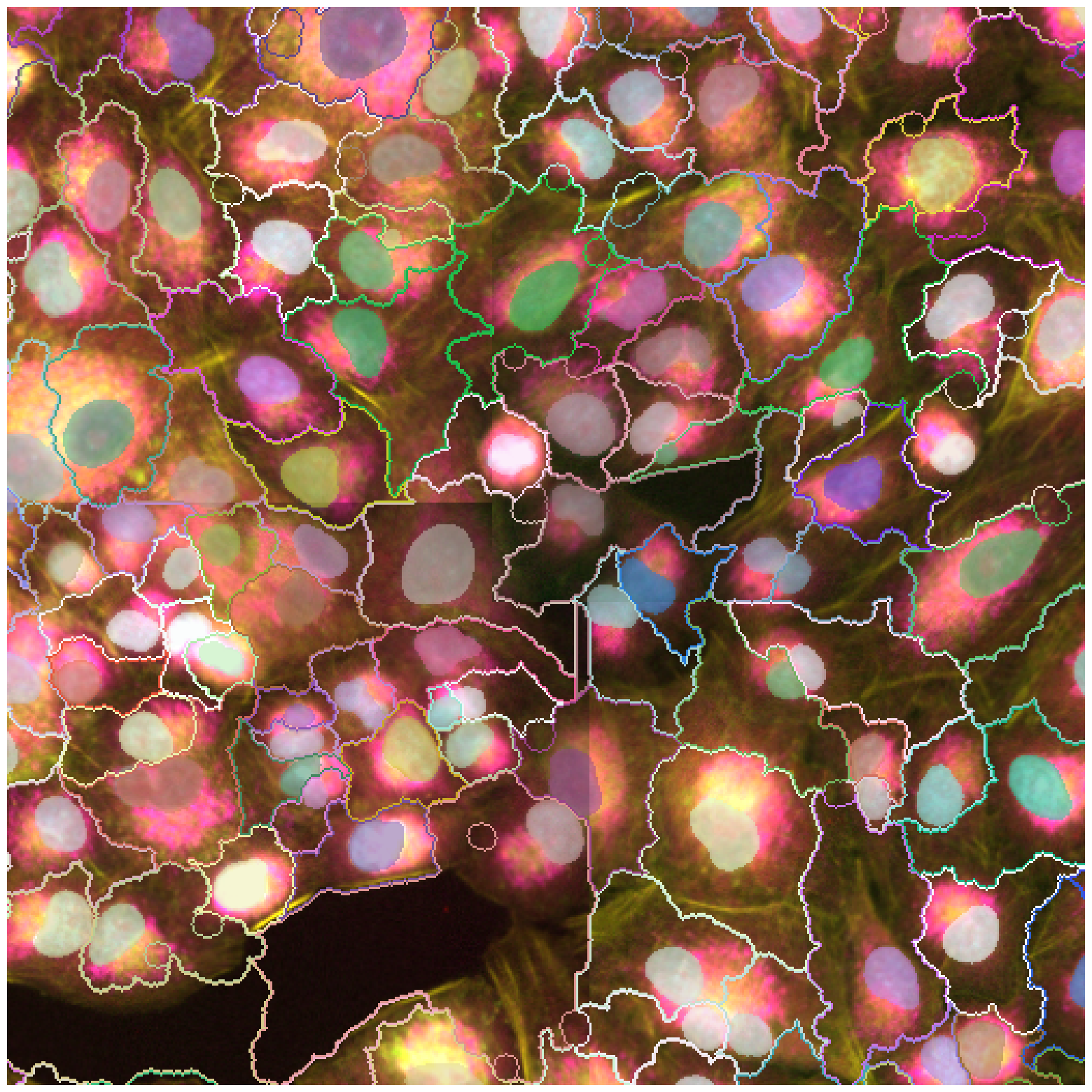
To evaluate physical traits at single-cell resolution, SCALLOPS isolates individual cells and subdivides them into distinct subcellular compartments: nuclei, cell bodies, and cytosols. The segmentation engine utilizes seed-propagated algorithms engineered to process massive image canvases out-of-core via Dask.

This process is split into two sequential steps:

Nuclei Segmentation: Automatically isolates nuclear boundaries across the plate using the DNA staining.
Cell Body Segmentation: Generates a high-contrast composite mask from all remaining channels to establish robust cell boundaries using the nuclear masks as initiation “seeds.”

Based on the PERISCOPE dataset structure, the five fluorescent channels map sequentially as 0-indexed values: DAPI=0, GFP=1, A594=2, Cy5=3, and 750=4. We target the DAPI signal at channel index 0 to isolate the nuclear boundaries.

Run the following command to generate your nuclear masks:

[6]:

scallops segment nuclei \
  --images "${OUTPUT_DIR}/stitch/pheno/stitch/stitch.zarr" \
  --groupby plate well \
  --image-pattern '{plate}-{well}' \
  --dapi-channel 0 \
  --output "${OUTPUT_DIR}/ops/segment.zarr" \
  --subset "${PLATE}-${WELL}"

06/02/2026 18:09 - Scallops version: 1.0.0
06/02/2026 18:09 - Scallops command:
scallops segment nuclei --images scallops_run/CP186A//stitch/pheno/stitch/stitch.zarr --groupby plate well --image-pattern {plate}-{well} --dapi-channel 0 --output scallops_run/CP186A//ops/segment.zarr --subset CP186A-1
06/02/2026 18:09 - Running nuclei segmentation for CP186A-1
WARNING: All log messages before absl::InitializeLog() is called are written to STDERR
I0000 00:00:1780423781.766639  327706 port.cc:153] oneDNN custom operations are on. You may see slightly different numerical results due to floating-point round-off errors from different computation orders. To turn them off, set the environment variable `TF_ENABLE_ONEDNN_OPTS=0`.
I0000 00:00:1780423781.820584  327706 cpu_feature_guard.cc:227] This TensorFlow binary is optimized to use available CPU instructions in performance-critical operations.
To enable the following instructions: AVX2 AVX512F AVX512_VNNI AVX512_BF16 FMA, in other operations, rebuild TensorFlow with the appropriate compiler flags.
WARNING: All log messages before absl::InitializeLog() is called are written to STDERR
I0000 00:00:1780423783.164239  327706 port.cc:153] oneDNN custom operations are on. You may see slightly different numerical results due to floating-point round-off errors from different computation orders. To turn them off, set the environment variable `TF_ENABLE_ONEDNN_OPTS=0`.
E0000 00:00:1780423783.550822  327706 cuda_platform.cc:52] failed call to cuInit: INTERNAL: CUDA error: Failed call to cuInit: UNKNOWN ERROR (303)
100%|█████████████████████████████████████████| 196/196 [02:10<00:00,  1.50it/s]
06/02/2026 18:16 - Processing done in 00H:06M:27S

By default this will use the method stardist (optionally can be cellpose) with its model 2D_versatile_fluo.

Once the nuclei are identified, we segment full cell boundaries. Rather than passing a single color wavelength, we supply all non-DAPI indexes (1 2 3 4) to the --cyto-channel argument. SCALLOPS dynamically aggregates these arrays to form a highly saturated composite cell mask, eliminating gaps caused by uneven marker expression. Note that if you have a dedicated channel for cell boundaries or you have a prefer channel, these can be used as well.

The underlying watershed or propagation algorithms use this composite canvas to trace cellular edges while maintaining a mathematically guaranteed one-to-one correspondence between nuclei seeds and cell labels.

(Note: Cytosol labels do not require a separate execution command; they are automatically computed downstream by taking the direct difference between the full cell masks and the nested nuclei masks.)

Run the following command to generate your cell body masks:

[3]:

scallops segment cell \
  --images "${OUTPUT_DIR}/stitch/pheno/stitch/stitch.zarr" \
  --groupby plate well \
  --image-pattern '{plate}-{well}' \
  --cyto-channel 1 2 3 4 \
  --nuclei-label "${OUTPUT_DIR}/ops/segment.zarr" \
  --output "${OUTPUT_DIR}/ops/segment.zarr" \
  --subset "${PLATE}-${WELL}" \
  --threshold "Local" \
  --sigma 1 \
  --closing-radius 5 \
  --force

06/03/2026 14:45 - Scallops version: 1.0.0
06/03/2026 14:45 - Scallops command:
scallops segment cell --images scallops_run/CP186A/stitch/pheno/stitch/stitch.zarr --groupby plate well --image-pattern {plate}-{well} --cyto-channel 1 2 3 4 --nuclei-label scallops_run/CP186A/ops/segment.zarr --output scallops_run/CP186A/ops/segment.zarr --subset CP186A-1 --threshold Local --sigma 1 --closing-radius 5 --force
06/03/2026 14:45 - Running cell segmentation for CP186A-1
06/03/2026 14:48 - Processing done in 00H:02M:46S

[4]:

python3 -c "
import matplotlib
matplotlib.use('Agg')
import matplotlib.pyplot as plt
import sys, os, warnings, logging

warnings.filterwarnings('ignore')
sys.stdout = open(sys.stdout.fileno(), mode='wb', buffering=0)

import numpy as np
from dask.distributed import Client
from scallops.io import read_experiment
from scallops.visualize.composite import imcomposite

size = 250
image = read_experiment('${OUTPUT_DIR}/stitch/pheno/stitch/stitch.zarr', dask=True).images['CP186A-1'].squeeze()
label = read_experiment('${OUTPUT_DIR}/ops/segment.zarr', dask=True)

y, x = np.array(image.shape[-2:]) // 2
yslice, xslice = slice(y - size, y + size), slice(x - size, x + size)

logging.getLogger('distributed').setLevel(logging.ERROR)

with Client(silence_logs=logging.ERROR):
    nuclei = label.labels['CP186A-1-nuclei'].isel(y=yslice, x=xslice).compute()
    cells = label.labels['CP186A-1-cell'].isel(y=yslice, x=xslice).compute()
    img = image.isel(y=yslice, x=xslice).compute()

fig, ax = plt.subplots(figsize=(20,20))
imcomposite(img, dim='c', figsize=(10, 10), labels_contour=cells, labels=nuclei, ax=ax)
ax.axis('off')

fig.savefig(sys.stdout, format='png', bbox_inches='tight')
sys.stdout.flush()
plt.close()
" | display

../_images/notebooks_End-to-End_31_0.png

With the sequencing (ISS) images registered to the baseline cycle ($t_0$) along Parallel Branch A, the next step is to detect the physical fluorescent puncta corresponding to individual sequenced transcript bases.

SCALLOPS locates these transcript spots across multiple imaging cycles by computing the standard deviation over the time (cycle) dimension, followed by the mean across the channels. If an experiment contains only a single imaging cycle, the engine adapts by calculating the standard deviation directly across the color channels instead. This spatial variance modeling allows SCALLOPS to separate static background cellular autofluorescence from true, dynamically shifting barcoding spots.

Run the following command to detect and map the coordinate arrays for all transcription spots across the plate:

[6]:

DASK_LOGGING__DISTRIBUTED=error scallops pooled-sbs spot-detect \
  --images "${OUTPUT_DIR}/ops/iss-registered-t0.zarr" \
  --image-pattern '{plate}-{well}' \
  --channel 1 2 3 4 \
  --output "${OUTPUT_DIR}/ops/spot-detect.zarr" \
  --groupby plate well \
  --subset "${PLATE}-${WELL}" \
  --force

06/03/2026 14:50 - Scallops version: 1.0.0
06/03/2026 14:50 - Scallops command:
scallops pooled-sbs spot-detect --images scallops_run/CP186A/ops/iss-registered-t0.zarr --image-pattern {plate}-{well} --channel 1 2 3 4 --output scallops_run/CP186A/ops/spot-detect.zarr --groupby plate well --subset CP186A-1 --force
06/03/2026 14:50 - Running spot detection for CP186A-1.
06/03/2026 15:03 - Processing done in 00H:13M:03S

Now that the transcript spot coordinates are mapped (from Parallel Branch A) and the cell segmentation boundaries are defined (from Parallel Branch B), the pipeline reaches its critical synchronization checkpoint.

In this step, SCALLOPS overlays the spot arrays directly onto the physical cellular or nuclei masks. The engine calculates the raw fluorescence intensities at each spot location across all sequencing cycles. Because the emission spectra of neighboring fluorescent dyes often overlap, SCALLOPS applies an algorithmic crosstalk correction to decouple the true signals. After correction, the base at each cycle is assigned to the channel exhibiting maximum intensity.

These raw base calls are assembled sequentially into a sequence string for each spot. SCALLOPS then cross-references these sequences against your experimental guide RNA codebook (--barcodes). It evaluates the alignment quality of each spot and calculates a Phred-scaled confidence score, outputting cleanly decoded single-guide RNA (sgRNA) tracking assignments tied to individual cells.

Run the following command to execute base calling and assign perturbation tracking barcodes across your cell masks:

[8]:

DASK_LOGGING__DISTRIBUTED=error scallops pooled-sbs reads \
  --spots "${OUTPUT_DIR}/ops/spot-detect.zarr" \
  --labels "${OUTPUT_DIR}/ops/segment.zarr" \
  --label-name nuclei \
  --barcodes "s3://cellpainting-gallery/cpg0021-periscope/broad/workspace/metadata/20200805_A549_WG_Screen/Barcodes.csv" \
  --barcode-col "sgRNA" \
  --output "${OUTPUT_DIR}/ops/reads" \
  --subset "${PLATE}-${WELL}" \
  --force

06/03/2026 15:13 - Scallops version: 1.0.0
06/03/2026 15:13 - Scallops command:
scallops pooled-sbs reads --spots scallops_run/CP186A/ops/spot-detect.zarr --labels scallops_run/CP186A/ops/segment.zarr --label-name nuclei --barcodes s3://cellpainting-gallery/cpg0021-periscope/broad/workspace/metadata/20200805_A549_WG_Screen/Barcodes.csv --barcode-col sgRNA --output scallops_run/CP186A/ops/reads --subset CP186A-1
06/03/2026 15:13 - Running reads for CP186A-1
06/03/2026 15:13 - Timepoint indices (0-based): 0, 1, 2, 3, 4, 5, 6, 7, 8, 9, 10, 11
06/03/2026 15:14 - 1,287,427 spots in labels.
06/03/2026 15:14 - Threshold peaks crosstalk correction: 125.12.
06/03/2026 15:14 - 65,093 spots in labels for crosstalk correction.
06/03/2026 15:14 - Computed crosstalk matrix.
06/03/2026 15:14 - Threshold peaks for assigning reads to labels: 23.10.
2026-06-03 15:15:06,780 - distributed.shuffle._scheduler_plugin - WARNING - Shuffle c551c7be2df5c678ffa5af2b9e1c0690 initialized by task ('shuffle-transfer-c551c7be2df5c678ffa5af2b9e1c0690', 0) executed on worker tcp://127.0.0.1:44465
2026-06-03 15:15:07,136 - distributed.shuffle._scheduler_plugin - WARNING - Shuffle c551c7be2df5c678ffa5af2b9e1c0690 deactivated due to stimulus 'task-finished-1780499707.1353924'
06/03/2026 15:16 - Processing done in 00H:02M:54S

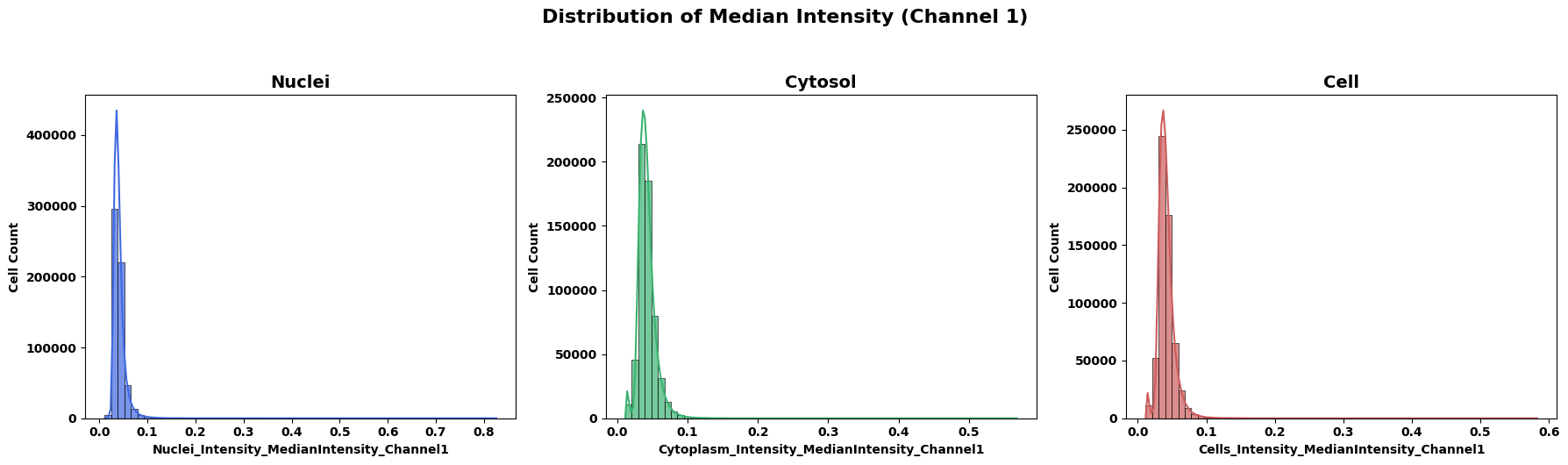
With our segmentation masks finalized, we transition to profiling the physical marker expressions of our cells. SCALLOPS extracts high-dimensional morphological and intensity data out-of-core via Dask, parsing our multi-scale OME Zarr canvas according to the spatial boundaries established in our segmentation file.

Rather than forcing you to compute spatial compartments sequentially, the scallops features CLI allows you to extract features for nuclei, cells, and cytosol simultaneously in a single command by supplying the --features-nuclei, --features-cell, and --features-cytosol arguments.

To keep our analysis highly optimized and focused exclusively on signal tracking, we will leverage the wildcard shortcut token: ``intensity_*``. This instructs the engine to dynamically loop through and extract intensity metrics across every individual 0-indexed channel present in the raw data (0 through 4), completely bypassing heavy structural texture algorithms, neighbor relations, or geometric metrics.

Production Optimization Note for Cluster Concurrency: While the features tool can isolate and discover discrete cellular objects automatically from your segmentation labels on the fly, doing so repeatedly during massive parallel cluster operations creates unnecessary computing overhead. When scaling up to mass concurrency across multi-node environments, it is best practice to run a standalone scallops find-objects pass once beforehand, and then pipe that cached directory to the optional --objects flag. Reusing those pre-computed static objects across concurrent feature worker nodes prevents redundant calculations, cuts down heavy S3 I/O bottlenecks, and significantly reduces cloud infrastructure costs.

Run the following terminal command to extract the channel intensity features across all three compartments at the same time:

[7]:

DASK_LOGGING__DISTRIBUTED=error scallops features \
  --images "${OUTPUT_DIR}/stitch/pheno/stitch/stitch.zarr" \
  --labels "${OUTPUT_DIR}/ops/segment.zarr" \
  --features-nuclei "intensity_*" \
  --features-cell "intensity_*" \
  --features-cytosol "intensity_*" \
  --output "${OUTPUT_DIR}/ops/features/" \
  --groupby 'plate' 'well' \
  --image-pattern '{plate}-{well}' \
  --subset "${PLATE}-${WELL}" \
  --force

06/03/2026 16:01 - Scallops version: 1.0.0
06/03/2026 16:01 - Scallops command:
scallops features --images scallops_run/CP186A/stitch/pheno/stitch/stitch.zarr --labels scallops_run/CP186A/ops/segment.zarr --features-nuclei intensity_* --features-cell intensity_* --features-cytosol intensity_* --output scallops_run/CP186A/ops/features/ --groupby plate well --image-pattern {plate}-{well} --subset CP186A-1 --force
06/03/2026 16:01 - Find cell objects for CP186A-1.
06/03/2026 16:06 - CP186A-1 cell 1 feature: intensity_*
06/03/2026 16:06 - Removed 0 out of 589,270 labels. Area: 21 to 969,590.
06/03/2026 16:06 - Number of channels: 5
06/03/2026 16:06 - Number of batches: 170
06/03/2026 16:07 - Find nuclei objects for CP186A-1.
06/03/2026 16:08 - CP186A-1 nuclei 1 feature: intensity_*
06/03/2026 16:08 - Removed 0 out of 589,270 labels. Area: 17 to 6,304.
06/03/2026 16:08 - Number of channels: 5
06/03/2026 16:08 - Number of batches: 1,423
06/03/2026 16:09 - Find cytosol objects for CP186A-1.
06/03/2026 16:14 - CP186A-1 cytosol 1 feature: intensity_*
06/03/2026 16:14 - Removed 18 out of 589,238 labels. Area: 2 to 969,157.
06/03/2026 16:14 - Number of channels: 5
06/03/2026 16:14 - Number of batches: 170
06/03/2026 16:15 - Processing done in 00H:14M:03S

[8]:

tree -L 2 "${OUTPUT_DIR}/ops/features/"

scallops_run/CP186A/ops/features/
├── cell
│   ├── CP186A-1-features.parquet
│   └── CP186A-1-objects.parquet
├── cytosol
│   ├── CP186A-1-features.parquet
│   └── CP186A-1-objects.parquet
└── nuclei
    ├── CP186A-1-features.parquet
    └── CP186A-1-objects.parquet

9 directories, 0 files

[12]:

python3 -c "
import pandas as pd
import matplotlib.pyplot as plt
import seaborn as sns
import sys, warnings
warnings.filterwarnings('ignore')
sys.stdout = open(sys.stdout.fileno(), mode='wb', buffering=0)
base_path = '${OUTPUT_DIR}/ops/features'
df_nuc = pd.read_parquet(f'{base_path}/nuclei/CP186A-1-features.parquet')
df_cyto = pd.read_parquet(f'{base_path}/cytosol/CP186A-1-features.parquet')
df_cell = pd.read_parquet(f'{base_path}/cell/CP186A-1-features.parquet')
def get_col(df):
    matches = [c for c in df.columns if 'MedianIntensity_Channel1' in c]
    return matches[0] if matches else None
fig, axes = plt.subplots(1, 3, figsize=(18, 5))
compartments = [
    (df_nuc, 'Nuclei', 'royalblue'),
    (df_cyto, 'Cytosol', 'mediumseagreen'),
    (df_cell, 'Cell', 'indianred')
]

for ax, (df, name, color) in zip(axes, compartments):
    col = get_col(df)
    if col:
        sns.histplot(df[col], bins=60, ax=ax, color=color, kde=True, edgecolor='black', alpha=0.7)
        ax.set_title(name, fontsize=14, weight='bold')
        ax.set_xlabel(col, fontsize=10)
        ax.set_ylabel('Cell Count', fontsize=10)
    else:
        ax.set_title(f'{name}\\n(Feature not found)', color='red')

plt.suptitle('Distribution of Median Intensity (Channel 1)', fontsize=16, weight='bold', y=1.05)
plt.tight_layout()

fig.savefig(sys.stdout, format='png', bbox_inches='tight')
plt.close()
" | display

../_images/notebooks_End-to-End_39_0.png

Now that the parallel branches have converged and completed execution, we have two primary outputs saved across our directory:

Phenotypic Data (from Parallel Branch B): Parquet files containing cellular compartment intensity metrics extracted across our target masks (/ops/features/).
Genetic Data (from Parallel Branch A): Decoded base calls and whitelist-filtered single-guide RNA (sgRNA) barcode tables (/ops/reads).

The final phase of the SCALLOPS pipeline is to execute a post-hoc consolidation and filtering routine. The pooled-sbs merge command functions as an automated dataset binder and quality-control filter. It maps every individual cell ID to its decoded barcode, merges the physical feature metrics, and cleans the final data matrix.

During this step, SCALLOPS evaluates the registration alignment between the moving sequencing cycles and the static phenotype morphology baseline using an integrated structural metric: ``correlation-pearson-box``.

This calculation computes the pixel-by-pixel Pearson correlation coefficient between key structural markers (such as the DAPI nuclear channel) inside a tight bounding box around each individual cell. If a cell exhibits an exceptionally low coefficient value, it indicates localized registration error or optical warping, allowing you to flag and filter out unstable cell measurements before downstream biological analysis.

Run the following terminal command to compile and QC your final dataset:

[5]:

scallops pooled-sbs merge \
  --sbs "${OUTPUT_DIR}/ops/reads/labels" \
  --output "${OUTPUT_DIR}/ops/merge/" \
  --barcodes "s3://cellpainting-gallery/cpg0021-periscope/broad/workspace/metadata/20200805_A549_WG_Screen/Barcodes.csv" \
  --barcode-col "sgRNA" \
  --phenotype "${OUTPUT_DIR}/ops/features/" \
  --subset "${PLATE}-${WELL}" \
  --force

06/03/2026 16:51 - Scallops version: 1.0.0
06/03/2026 16:51 - Scallops command:
scallops pooled-sbs merge --sbs scallops_run/CP186A/ops/reads/labels --output scallops_run/CP186A/ops/merge/ --barcodes s3://cellpainting-gallery/cpg0021-periscope/broad/workspace/metadata/20200805_A549_WG_Screen/Barcodes.csv --barcode-col sgRNA --phenotype scallops_run/CP186A/ops/features/ --subset CP186A-1 --force
06/03/2026 16:51 - Running merge for CP186A-1 with /home/ubuntu/scallops/docs/notebooks/scallops_run/CP186A/ops/features/cell/CP186A-1-features.parquet, /home/ubuntu/scallops/docs/notebooks/scallops_run/CP186A/ops/features/cell/CP186A-1-objects.parquet, /home/ubuntu/scallops/docs/notebooks/scallops_run/CP186A/ops/features/cytosol/CP186A-1-features.parquet, /home/ubuntu/scallops/docs/notebooks/scallops_run/CP186A/ops/features/cytosol/CP186A-1-objects.parquet, /home/ubuntu/scallops/docs/notebooks/scallops_run/CP186A/ops/features/nuclei/CP186A-1-features.parquet, /home/ubuntu/scallops/docs/notebooks/scallops_run/CP186A/ops/features/nuclei/CP186A-1-objects.parquet.
06/03/2026 16:51 - Timepoint indices (0-based): 0, 1, 2, 3, 4, 5, 6, 7, 8, 9, 10, 11
06/03/2026 16:51 - Removed 1 duplicate barcode
06/03/2026 16:51 - Processing done in 00H:00M:16S

[7]:

tree -L 2 ${OUTPUT_DIR}/ops/merge/

scallops_run/CP186A/ops/merge/
└── CP186A-1.parquet

0 directories, 1 file

You have successfully walked through an end-to-end processing pipeline using the SCALLOPS CLI on the PERISCOPE dataset.

By executing these steps, your raw, unstructured multi-channel .nd2 image files have been fully standardized, stitched, aligned across cycles, segmented into discrete cells, base-called, profiled for physical traits, and merged into a clean, analysis-ready feature matrix.

You can now load your consolidated Parquet and CSV files from the ${OUTPUT_DIR}/results/ workspace straight into downstream analytical environments (such as Scanpy, Pandas, or R) to map precise phenotypes directly to genetic perturbations.