Optical Pooled Screening Example

Before starting any full scale experiment, it is always recommended to explore a few tiles such that thresholds are set, segmentation is evaluated and in general have a better understanding of the data. This notebook walks you through some of the steps that you can use to do such a task

Load Experiment

The first step in any pipeline is to load the experiment. SCALLOPS can load single image with read_image, or an entire experiment (or a subset if requested) with read_experiment:

from scallops.datasets import feldman_2019_small
from scallops.io import read_experiment

experiment_c_path = feldman_2019_small()
image_path = experiment_c_path / "input"
image_pattern = "{prefix}/{mag}X_c{t}-{experiment}-{t}_{well}_Tile-{tile}.{datatype}.tif"  # Pattern that is followed by the images

In this particular example we will use several tiles of the public dataset experiment C. Its directory structure is (from the input directory):

├── 10X_c1-SBS-1
│   ├── 10X_c1-SBS-1_A1_Tile-102.sbs.tif
│   └── 10X_c1-SBS-1_A1_Tile-103.sbs.tif
├── 10X_c10-SBS-10
│   ├── 10X_c10-SBS-10_A1_Tile-102.sbs.tif
│   └── 10X_c10-SBS-10_A1_Tile-103.sbs.tif
├── 10X_c2-SBS-2
│   ├── 10X_c2-SBS-2_A1_Tile-102.sbs.tif
│   └── 10X_c2-SBS-2_A1_Tile-103.sbs.tif
├── 10X_c3-SBS-3
│   ├── 10X_c3-SBS-3_A1_Tile-102.sbs.tif
│   └── 10X_c3-SBS-3_A1_Tile-103.sbs.tif
├── 10X_c4-SBS-4
│   ├── 10X_c4-SBS-4_A1_Tile-102.sbs.tif
│   └── 10X_c4-SBS-4_A1_Tile-103.sbs.tif
├── 10X_c5-SBS-5
│   ├── 10X_c5-SBS-5_A1_Tile-102.sbs.tif
│   └── 10X_c5-SBS-5_A1_Tile-103.sbs.tif
├── 10X_c7-SBS-7
│   ├── 10X_c7-SBS-7_A1_Tile-102.sbs.tif
│   └── 10X_c7-SBS-7_A1_Tile-103.sbs.tif
├── 10X_c8-SBS-8
│   ├── 10X_c8-SBS-8_A1_Tile-102.sbs.tif
│   └── 10X_c8-SBS-8_A1_Tile-103.sbs.tif
└── 10X_c9-SBS-9
    ├── 10X_c9-SBS-9_A1_Tile-102.sbs.tif
    └── 10X_c9-SBS-9_A1_Tile-103.sbs.tif

that is 9 cycles (missing cycle #6) of SBS data in two tiles of the well A1. The pattern that we have provided above ({prefix}/{mag}X_c{t}-{experiment}-{t}_{well}_Tile-{tile}.{datatype}.tif) contains:

1. prefix: this will store any parent directory name, e.g. 10X_c8-SBS-8, etc.

2. mag: Will store only the integer part of the magnification, 10 in this case.

3. t: Will store the t dimension. Since this is SBS data, it constitutes the cycle information.

4. experiment: The type of experiment.

5. well: from which well it comes from.

6. tile: which tile we are dealing with.

7. datatype: which kind of data it is. In this case, sbs.

All of these patterns can be arbitrary names that makes sense to you with the exception of the t, c, or z handles, as SCALLOPS will look for this name to store it appropriately.

Now that we know the structure of our data, let’s read it:

iss_experiment = read_experiment(image_path, image_pattern, group_by=("well", "tile"))
print(iss_experiment)
print(iss_experiment.images.keys())
print(
    read_experiment(
        image_path, image_pattern, group_by=("well", "tile"), subset=["A1-102"]
    )
)  # If you want to subset your experiment

Experiment with 2 images and 0 labels
dict_keys(['A1-102', 'A1-103'])
Experiment with 1 image and 0 labels

Now we have our experiment loaded and ready to go. Now let’s access some images, and deal with the barcodes.

Load ISS Image and Barcodes

For some of the examples we will show you, we will use the image A1-102 as key. For experiment C the order of the bases was G, T, A C, and the dapi channel was capture first (index 0). All these parameters are important to do some of the processing of the data:

import numpy as np

from scallops.io import read_barcodes

image_key = "A1-102"  # Set the image key
dapi_channel = 0  # set a single dapi channel index
barcodes_path = experiment_c_path / "barcodes.csv"

iss_image = iss_experiment.images[image_key].max(
    dim="z", keep_attrs=True
)  # Get the image, and use the max z if any exist
iss_channels = np.delete(
    np.arange(iss_image.sizes["c"]), dapi_channel
)  # get the ISS only channels (remove dapi)
df_barcode = read_barcodes(
    barcodes_path, iss_image.t.values - 1
)  # Read the barcodes using the actual t indexes (missing cycle 6)
print("Image dimensions:", iss_image.sizes)
df_barcode.head()

Image dimensions: Frozen({'t': 9, 'c': 5, 'y': 1024, 'x': 1024})

	barcode	sgRNA	gene_symbol
0	CATTGACGC	CATTGCACGCCACAGCATTG	non-targeting
1	GAGTTCTAG	GAGTTTCTAGTAGTGGTAGG	non-targeting
2	AACGCGTCG	AACGCTGTCGTACGTGTATA	non-targeting
3	GCGGGCGGT	GCGGGGCGGTGACTTTCAAG	non-targeting
4	TTCTAGCCA	TTCTAAGCCACGTGTGGTAC	non-targeting

Note that the barcodes contain all cycles except 6, as we expected. The read_barcodes is a utility simple function that also allows you to have a different name for the barcode by passing the barcode_column argument.

ISS Image

Now that we have a single image loaded into memory (iss_image), it is time to explore how it looks. There are a number of things that you might want to check, starting with what your data looks like in each channel. Luckily SCALLOPS’ plotting submodules will help with that. Let’s start with a montage plot of the channels with montage_plot:

from scallops.visualize.composite import montage_plot

montage_plot(iss_image)

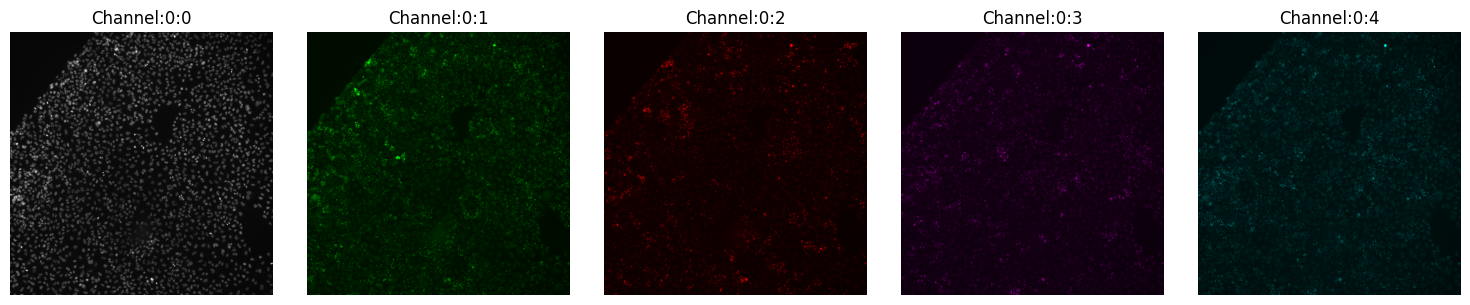
The figure above shows you every channel and you can make inferences about the quality, etc. However, it tells us very little about the alignment of the channels. During capture, channels and cycles can get misaligned, and that can create issues for downstream analyses.

Registration

The act of aligning channels and cycles is called registration. This is a crucial step, as it will be needed for base calling, etc. But before we go to the registration functions, let’s first verify how badly mis-aligned things are. SCALLOPS provides two ways to check this: imcomposite and diagnose_registration.

imcomposite

This shows a composite of all channels in a single image over a particular dimension. It is the most flexible and complete function for this task:

from scallops.visualize.composite import imcomposite

imcomposite(iss_image.isel(c=dapi_channel), dim="t", figsize=(10, 10));

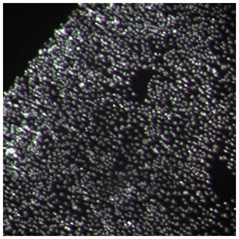
Here you can clearly see misalignment.

diagnose_registration

The other lightweight option is called diagnose_registration which is a simpler function. It has more limitations (only up to 6 images can be combined), but provides a bit more contrast than the imcomposite:

import matplotlib.pyplot as plt

from scallops.visualize.registration import diagnose_registration

# Let's get some selectors
selectors = [
    {"t": 1, "c": "Channel:0:0"},  # DAPI in first cycle
    {"t": 1, "c": "Channel:0:1"},  # G in first cycle
    {"t": 1, "c": "Channel:0:2"},  # T in first cycle
    {"t": 1, "c": "Channel:0:3"},  # A in first cycle
    {"t": 1, "c": "Channel:0:4"},  # C in first cycle
    {"t": 2, "c": "Channel:0:0"},  # DAPI in second cycle
]
f, ax = plt.subplots(figsize=(10, 10))
axes = diagnose_registration(iss_image, *selectors, title="Before alignment")

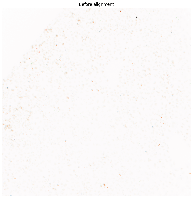
The reason for the cap in the number of selectors is to keep the colormaps more dissimilar.

Both above cases showed us that the cycles and channels are not fully aligned, and we need to deal with this. This process is called registration. You can register an images with align_image:

from scallops.registration.crosscorrelation import align_image

iss_image = align_image(
    iss_image,
    align_within_time_channels=iss_channels,  # Ensure we align all channels within a cycle
    align_between_time_channel=dapi_channel,  # Ensure we align all cycles
    filter_percentiles=[0, 90],  # reduces potential noise during aligning (is optional)
)
imcomposite(iss_image.isel(c=dapi_channel), dim="t", figsize=(10, 10));

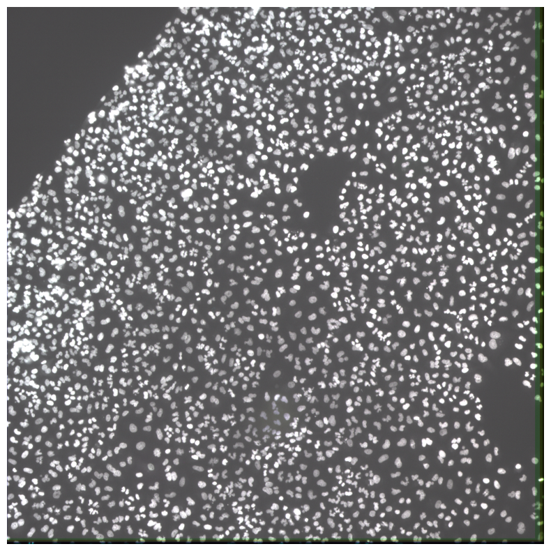
Now our ISS image is aligned.

Segmentation

The next step after registration is to segment the cellular compartments, starting with nuclei. SCALLOPS provides multiple algorithms for segmentation.

Segment Nuclei

Most OPS experiments start with segementing the nuclei. In fact most of our cellular segmentation options are seeded with the nuclear mask. For this tutorial we will focus on the stardist method, as we find it usually gives a good segmentation. That being said, the proper segmentation algorithm is very dataset dependent, so we encourage you to explore multiple algorithms. In SCALLOPS, stardist nuclear segmentation is called segment_nuclei_stardist.

from scallops.segmentation.stardist import segment_nuclei_stardist

all_nuclei = segment_nuclei_stardist(image=iss_image, nuclei_channel=dapi_channel)
print(f"Nuclei, {len(np.unique(all_nuclei)) - 1:,}")

bioimageio_utils.py (2): pkg_resources is deprecated as an API. See https://setuptools.pypa.io/en/latest/pkg_resources.html. The pkg_resources package is slated for removal as early as 2025-11-30. Refrain from using this package or pin to Setuptools<81.
tf2onnx_lib.py (8): In the future `np.object` will be defined as the corresponding NumPy scalar.

Nuclei, 2,968

After acquiring the nuclei mask we would like to:

1. Visualize the mask

2. Check some geometric features

These two steps will help you verify and filter potential artifact of bad segmented areas, and define thresholds. For the first one we can use imcomposite again:

imcomposite(
    iss_image.isel(c=dapi_channel), dim="t", figsize=(10, 10), labels_contour=all_nuclei
);

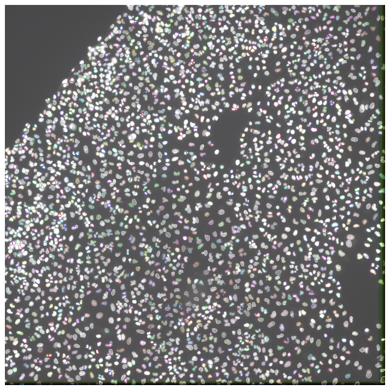
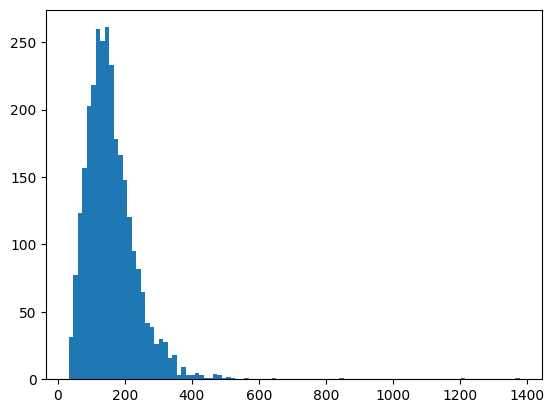
Now lets look at the distribution of nuclei areas and set some thresholds. To extract this feature we will be using skimage.measure.regionprops_table:

from skimage.measure import regionprops_table

nuclei_props = regionprops_table(all_nuclei, properties=["area"])
plt.hist(nuclei_props["area"], bins=100);

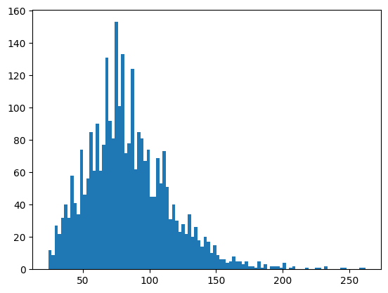
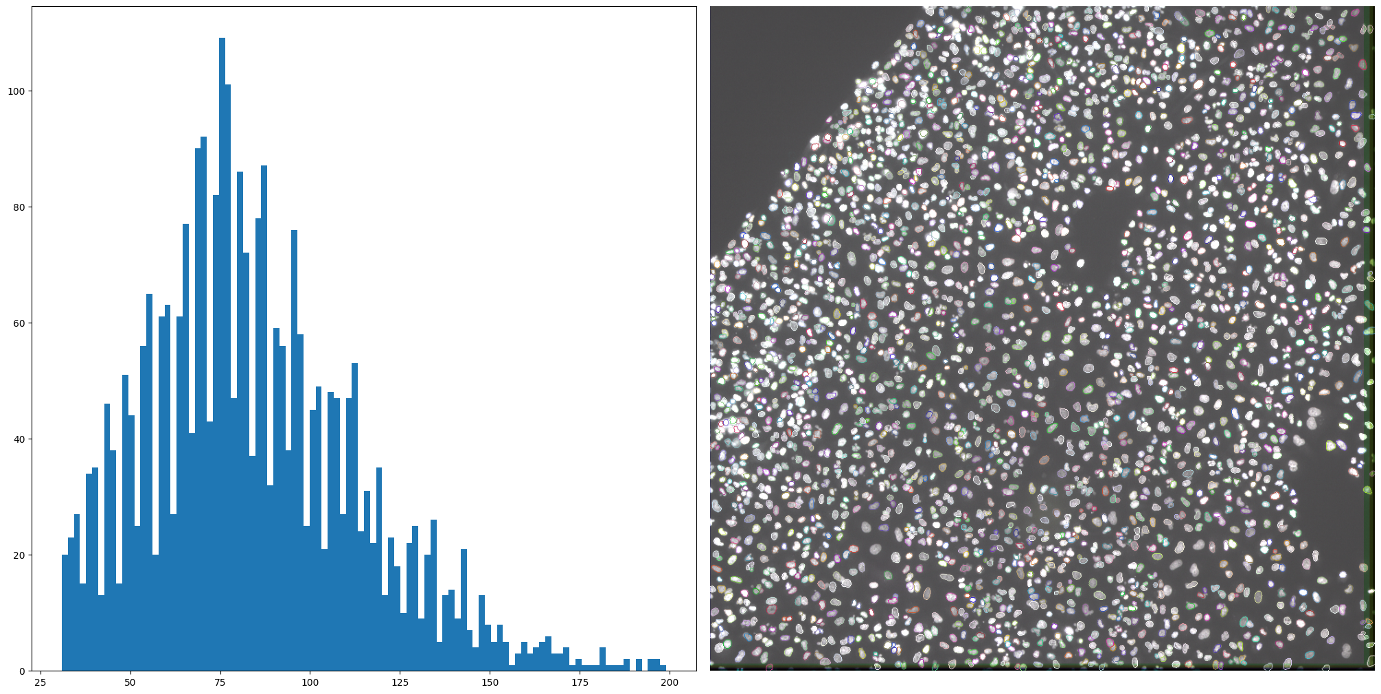
The distribution shows us a long tail, which is something that you would want to be inspected. From the visualization we can also see that there are a set of nuclei that seem too small. For the purposes of this example, we will assume that objects smaller than 30 and bigger than 200 are either artifacts, cells in mitotic state, or in general something we would like to filter out. SCALLOPS has a utility function filter_labels_by_area:

from scallops.segmentation.util import remove_labels_by_area

nuclei_area_min = 30
nuclei_area_max = 200
nuclei = remove_labels_by_area(all_nuclei, nuclei_area_min, nuclei_area_max)
nuclei_props = regionprops_table(nuclei, properties=["area"])
f, axs = plt.subplots(ncols=2, figsize=(20, 10), layout="constrained")
axs[0].hist(nuclei_props["area"], bins=100)
imcomposite(iss_image.isel(c=dapi_channel), dim="t", labels_contour=nuclei, ax=axs[1]);

Segment cells

Now that we nuclei, we segment the cells. In some datasets, we found that given good nuclei seeds, watershed does an good job in segmenting the cells if the cell staining channel is well saturated. For this example we will be using segment_cells_watershed. In order to so, however, we do need to provide a threshold. There are a number of automatic algorithms available in this function (see API), but for simplicity we will pass a single threshold value. To do this, we need to explore the distribution of the intensities, including and excluding nuclei. Since our data so far is ISS, we do not have a cytosolic channel (such as ConA for example). In these cases, we can create an average mask by using SCALLOPS’ function cyto_channel_summary:

from scallops.segmentation.util import cyto_channel_summary

cell_mask = cyto_channel_summary(
    iss_image.isel(t=0, c=iss_channels)
)  # get an average mask for cells
f, ax = plt.subplots(figsize=(6, 6))
cell_mask_clipped = cell_mask.clip(
    max=cell_mask.quantile(0.98)
)  # Avoid really bright spots
in_nuc = cell_mask_clipped.data[nuclei > 0].flatten()  # Get values in nuclei
out_nucl = cell_mask_clipped.data[nuclei == 0].flatten()  # Get values outside nuclei
ax.boxplot([in_nuc, out_nucl], tick_labels=["In Nuclei", "Not in Nuclei"])
ax.set_ylabel("Intensity in Cell Mask");

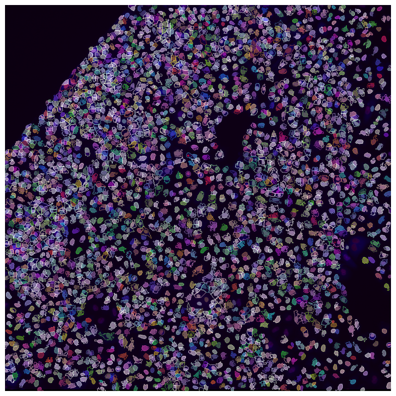
Judging by the above plot we set the cell threshold to 650:

from scallops.segmentation.watershed import segment_cells_watershed

cell_segmentation_threshold = 650  # Set the threshold
all_cells, _ = segment_cells_watershed(
    iss_image, nuclei, threshold=cell_segmentation_threshold
)  # segment the cells
imcomposite(
    iss_image.isel(c=dapi_channel),
    dim="t",
    labels=nuclei,  # visualize nuclei solid
    labels_contour=all_cells,  # visualize cells as boundaries
    figsize=(10, 10),
)
plt.title(f"Cells, {len(np.unique(all_cells)) - 1:,}");

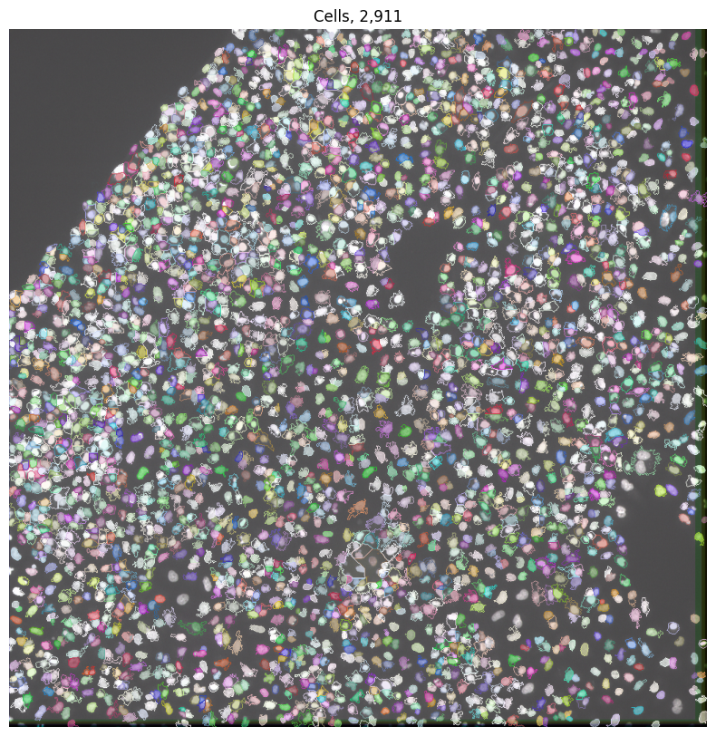
We can see a pretty good segmentation (despite some holes and lack of definition here and there) given that there is no cytosolic mask. Let us assume that this segmentation is good, and lets clean it up a little. Similar to the nuclei, we can visualize and inspect the cellular area, and then filter based on set thresholds:

cell_props = regionprops_table(all_cells, properties=["area"])
plt.hist(cell_props["area"], bins=100);

Now we can set the minimum and maximum areas allowed to 40 and 500:

cell_area_min = 40
cell_area_max = 500
cells = remove_labels_by_area(all_cells, cell_area_min, cell_area_max)
cell_props = regionprops_table(cells, properties=["area"])
fig, axes = plt.subplots(1, 2, figsize=(10, 5), layout="constrained")
axes[0].set_title("Cell Area")
axes[0].hist(cell_props["area"], bins=100)
axes[1].set_title(f"Cells, {len(np.unique(cells)) - 1:,}")
imcomposite(image=iss_image.isel(c=dapi_channel), dim="t", labels=cells, ax=axes[1])
axes[1].axis("off");

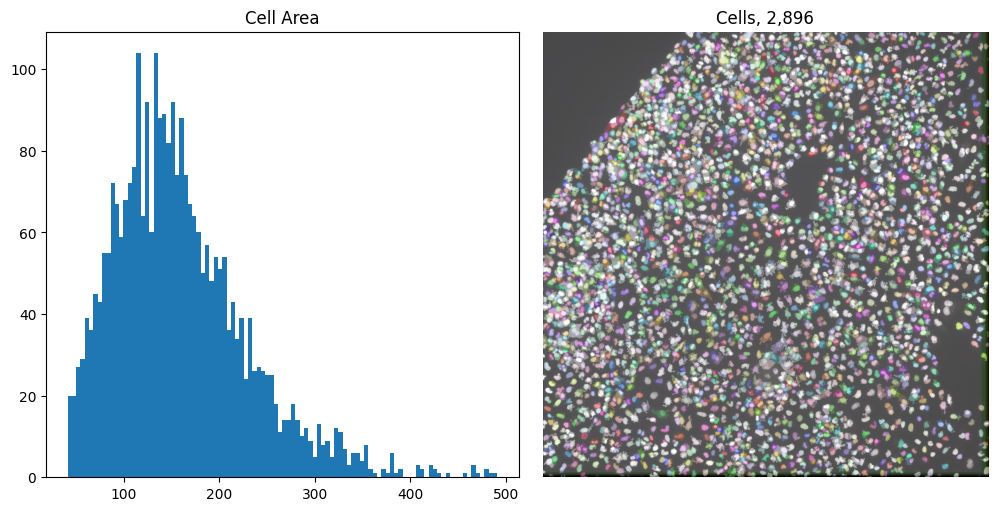
Now we have both cells and nuclei segmented, we can move to barcode calling.

Barcode calling

In OPS to call the barcodes we need to:

1. Find peaks: Identify the intensity peaks that are shared across all ISS channels

2. Filter peaks: Identify false positive and filter them

3. Cross-talk correction: Compute the cross-talk and corrected

4. Call Bases: Based on the max corrected intensities in each cycle, call the bases

5. Call reads: Call reads by calling the base with the highest intensity

Find Peaks

Finding the peaks requires to denoise the image with Laplacian of Gaussian (LoG) transform, followed by computing the standard deviation across sequencing channels, to identify where peaks are. This can be done with transform_log, std, and find_peaks, respectively:

from scallops.spots import find_peaks, std, transform_log

loged = transform_log(iss_image.isel(c=iss_channels))
std_arr = std(loged)
peaks = find_peaks(std_arr)
bases_array = find_peaks(std_arr)

Call Bases

To call bases we need to compute the maximum filter over the LoG transform using the max_filter function followed by the calling function peaks_to_bases:

from scallops.reads import peaks_to_bases
from scallops.spots import max_filter

maxed = max_filter(loged)
bases_array = peaks_to_bases(maxed=maxed, peaks=peaks, labels=cells)
bases_array.sizes

Frozen({'read': 10557, 't': 9, 'c': 4})

Now we have all unfiltered peaks. We divide the unfiltered peaks into high quality and low quality peaks by computing the probability of the bases in the read at the peak location. We choose the peak threshold with the maximimum F0.5 score using . peak_thresholds_from_bases

from scallops.spots import peak_thresholds_from_bases

threshold_peaks_crosstalk_correction_df = peak_thresholds_from_bases(
    bases_array=bases_array
)
threshold_peaks_crosstalk_correction = threshold_peaks_crosstalk_correction_df.iloc[0][
    "threshold"
]

f"Crosstalk peak threshold: {threshold_peaks_crosstalk_correction}"

'Crosstalk peak threshold: 103.40227203832168'

Cross-talk correction

Now we can visualize the cross-talk with pairwise_channel_scatter_plot:

from scallops.visualize.crosstalk import pairwise_channel_scatter_plot

fig, _ = pairwise_channel_scatter_plot(
    bases_array.where(
        bases_array.peak > threshold_peaks_crosstalk_correction, drop=True
    )
)
fig.suptitle("Uncorrected Intensity (In Cells)")
fig.tight_layout()

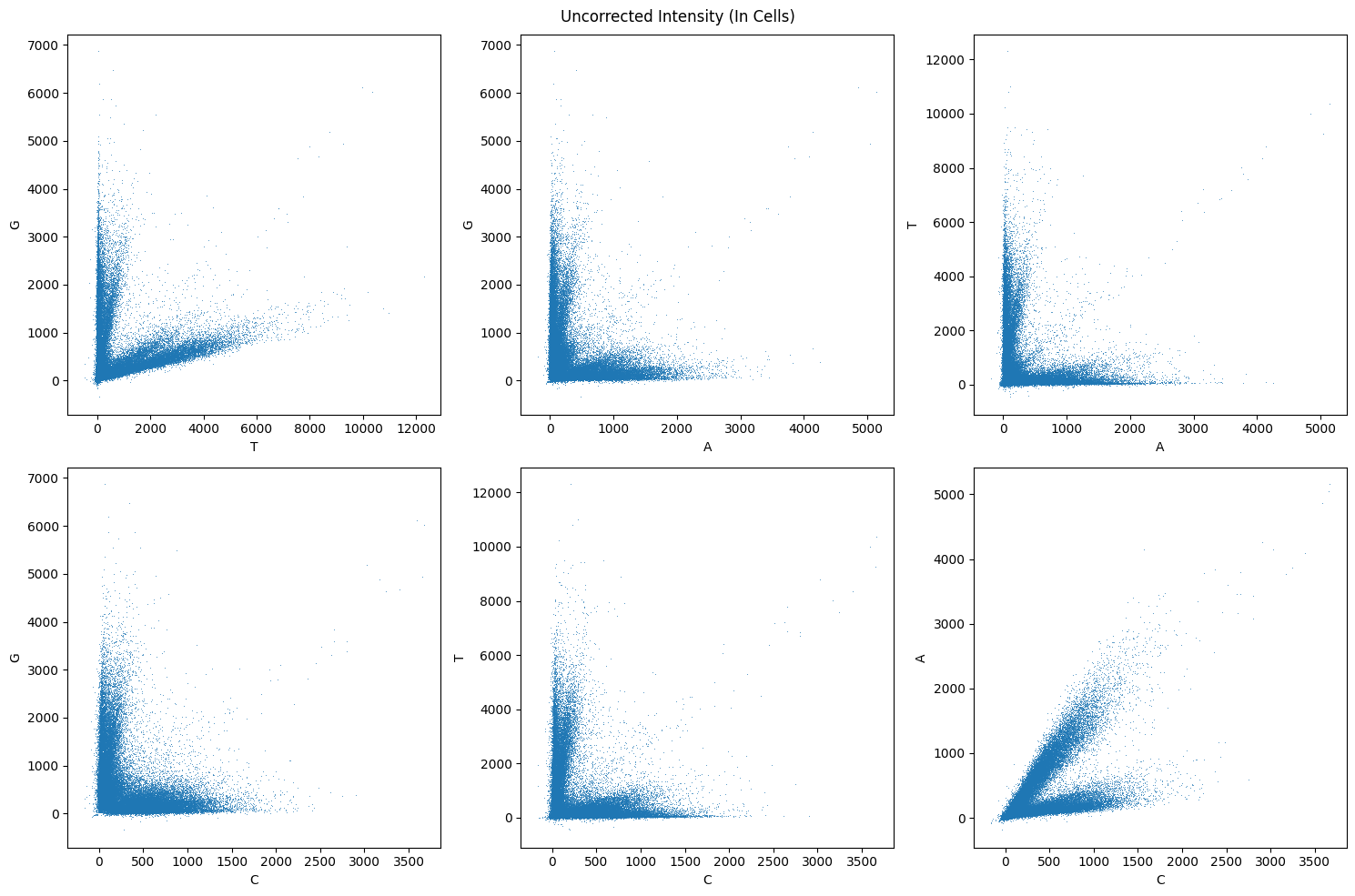
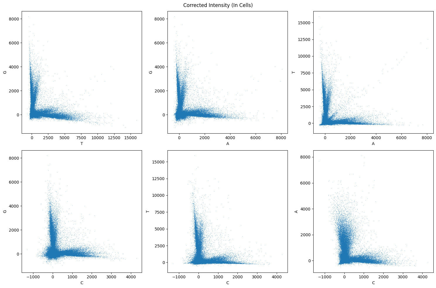
We can see that there is some cross-talk, especially betwen A and C and T and G. Now we need to compute the cross-talk matrix with channel_crosstalk_matrix, correct the cross-talk with apply_channel_crosstalk_matrix, and again visualize the result of the correction.

from scallops.reads import apply_channel_crosstalk_matrix, channel_crosstalk_matrix

w = channel_crosstalk_matrix(
    bases_array.where(
        bases_array.peak > threshold_peaks_crosstalk_correction, drop=True
    )
)
corrected_bases_array = apply_channel_crosstalk_matrix(bases_array, w)
fig, _ = pairwise_channel_scatter_plot(corrected_bases_array)
fig.suptitle("Corrected Intensity (In Cells)")
fig.tight_layout()

Call Reads

Now that we have a corrected set of base intensities, we can call the reads using SCALLOPS’ decode-max function, and we can see some descriptive read statistics with read_statistics:

from scallops.reads import decode_max, read_statistics
from scallops.spots import peak_thresholds_from_reads

df_reads = decode_max(corrected_bases_array, barcodes=df_barcode)
peak_thresholds_lower_df = peak_thresholds_from_reads(df_reads.query("barcode_match"))
threshold_peaks = peak_thresholds_lower_df.iloc[0]["threshold"]
f"Lower peak threshold: {threshold_peaks:.2f}"

'Lower peak threshold: 49.46'

df_reads = df_reads.query(f"peak>{threshold_peaks}")
read_statistics(df_reads)

{'mapped_reads': 5981,
 'number_of_reads': 7632,
 'mapping_rate': 0.7836740041928721,
 'mapping_rate_within_labels': 0.7836740041928721,
 'mapped_reads_within_labels': 5981,
 'average_reads_per_label': 3.0974025974025974,
 'average_mapped_reads_per_label': 2.427353896103896,
 'number_of_unique_barcodes_in_labels': 825,
 'mean_barcode_count_in_labels': 7.24969696969697,
 'labels_with_reads': 2464,
 'labels_with_mapped_reads': 2202}

Visualize Single Base Calling Errors

After base calling we want to visualize the biases and mismatches across our bases. We can obtain the summary of the mismatches using SCALLOPS’ summarize_base_call_mismatches, and then visualize with base_call_mismatches_heatmap:

from scallops.reads import summarize_base_call_mismatches
from scallops.visualize.heatmap import base_call_mismatches_heatmap

base_call_mismatches_df = summarize_base_call_mismatches(df_reads, df_barcode)
display(base_call_mismatches_df.head())
base_call_mismatches_heatmap(base_call_mismatches_df);

	called_base	whitelist_base	read_position	count	fraction
0	A	C	0	2	0.003868
1	A	C	1	2	0.003868
2	A	C	2	2	0.003868
3	A	C	3	2	0.003868
4	A	C	4	8	0.015474

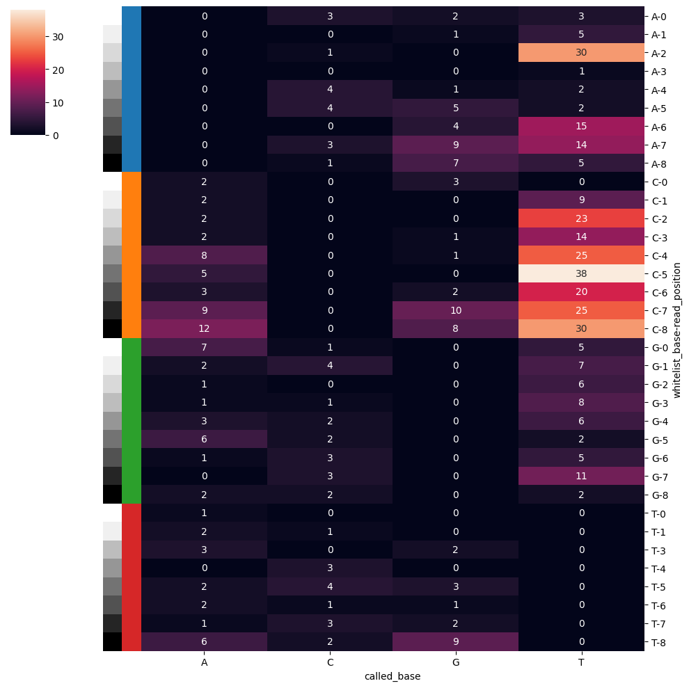
Correct Reads With One Mismatch

The figure above showed us that there are mismatches from our expected barcode list. We can try fliping bases to match the whitelist. This can be done by computing the hamming distance and restricting the flipping to a desired number of mismatches you want fixed. This can easily be achieved by SCALLOPS’ correct_mismatches function:

from scallops.reads import correct_mismatches

df_reads = correct_mismatches(df_reads, df_barcode)
read_statistics(df_reads)

{'mapped_reads': 6498,
 'number_of_reads': 7632,
 'mapping_rate': 0.8514150943396226,
 'mapping_rate_within_labels': 0.8514150943396226,
 'mapped_reads_within_labels': 6498,
 'average_reads_per_label': 3.0974025974025974,
 'average_mapped_reads_per_label': 2.637175324675325,
 'number_of_unique_barcodes_in_labels': 949,
 'mean_barcode_count_in_labels': 6.847207586933615,
 'labels_with_reads': 2464,
 'labels_with_mapped_reads': 2297}

df_reads.head()

	y	x	sigma	peak	label	read	barcode	Q	Q_mean	Q_min	barcode_match	mismatches	closest_match	mismatches2	closest_match2	barcode_uncorrected
19	5	756	1	1189.094209	924	19	AAGCCAATT	[60.0, 60.0, 60.0, 60.0, 60.0, 60.0, 60.0, 60....	60.0	60.0	True	NaN	NaN	NaN	NaN	NaN
20	5	791	1	488.943090	2258	20	AGCATGCCA	[60.0, 60.0, 60.0, 60.0, 60.0, 60.0, 60.0, 60....	60.0	60.0	True	NaN	NaN	NaN	NaN	NaN
21	5	796	1	372.566588	2258	21	AGCATGCCA	[60.0, 60.0, 60.0, 60.0, 60.0, 60.0, 60.0, 60....	60.0	60.0	True	NaN	NaN	NaN	NaN	NaN
22	5	809	1	187.319520	2258	22	AAGAGTTCT	[60.0, 60.0, 60.0, 60.0, 60.0, 60.0, 60.0, 60....	60.0	60.0	True	NaN	NaN	NaN	NaN	NaN
39	6	481	1	58.776617	1506	39	AAGGGGTCT	[60.0, 60.0, 60.0, 60.0, 60.0, 60.0, 60.0, 60....	60.0	60.0	False	1.0	AAGGCGTCT	1.0	AAGGGCTCT	NaN

Our overall mapping rate is now higher and we also find more cells with mapped reads than before the correction.

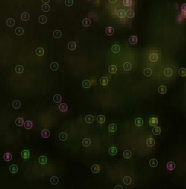
Interactive visualization of Base Calls

We can use Napari to interactively visualize the base calls and the underlying data with SCALLOPS’ add_bases:

import napari

from scallops.visualize.napari import add_bases

viewer = napari.Viewer()
viewer.add_image(
    iss_image.squeeze(),
    channel_axis=1,
    visible=[False, True, True, True, True],
    name=["DAPI"] + ["G", "T", "A", "C"],
)
add_bases(viewer, df_reads)
viewer.add_labels(
    cells,
    name="cells",
    colormap=napari.utils.DirectLabelColormap(color_dict={None: (1, 1, 1, 0.5)}),
).contour = 1

The above code should open a new window with napari, and the bases should be in the left-hand side panel. A zoom in should look like this:

Assign Barcodes To Cells

So far we have successfully called the barcodes, but we still need to assign the barcode to each label. This can be achieved by calling assign_barcodes_to_labels:

from scallops.reads import assign_barcodes_to_labels

df_cells = assign_barcodes_to_labels(df_reads).set_index("label")
df_cells

	mismatch	barcode_Q_mean	barcode_Q_min	barcode_peak	barcode_count	barcode_0	barcode_Q_mean_0	barcode_Q_min_0	barcode_peak_0	barcode_count_0	barcode_Q_0	barcode_1	barcode_Q_mean_1	barcode_Q_min_1	barcode_peak_1	barcode_count_1	barcode_Q_1
label
924	False	60.000000	60.000000	1189.094209	1	AAGCCAATT	60.000000	60.000000	1189.094209	1	[60.0, 60.0, 60.0, 60.0, 60.0, 60.0, 60.0, 60....		0.000000	0.000000	NaN	0	None
2258	False	300.000000	300.000000	1801.712283	5	AGCATGCCA	180.000000	180.000000	1479.391942	3	[180.0, 180.0, 180.0, 180.0, 180.0, 180.0, 180...	AAGAGTTCT	60.000000	60.000000	187.319520	1	[60.0, 60.0, 60.0, 60.0, 60.0, 60.0, 60.0, 60....
1506	True	60.000000	60.000000	58.776617	1	AAGGGGTCT	60.000000	60.000000	58.776617	1	[60.0, 60.0, 60.0, 60.0, 60.0, 60.0, 60.0, 60....		0.000000	0.000000	NaN	0	None
2900	False	120.000000	120.000000	1040.681147	2	AAGCCAATT	120.000000	120.000000	1040.681147	2	[120.0, 120.0, 120.0, 120.0, 120.0, 120.0, 120...		0.000000	0.000000	NaN	0	None
2664	False	238.460434	226.906937	1075.447078	4	TCCATTGCA	238.460434	226.906937	1075.447078	4	[240.0, 226.90694, 240.0, 240.0, 240.0, 240.0,...		0.000000	0.000000	NaN	0	None
...	...	...	...	...	...	...	...	...	...	...	...	...	...	...	...	...	...
1291	True	106.944305	2.498775	1709.110210	2	TTTGGGCAG	53.472153	1.249387	1355.472936	1	[60.0, 60.0, 60.0, 60.0, 60.0, 60.0, 60.0, 60....	GGGGTGCAG	53.472153	1.249387	353.637274	1	[60.0, 60.0, 60.0, 60.0, 60.0, 60.0, 60.0, 60....
2826	True	53.472153	1.249387	87.979374	1	ACAACCCAG	53.472153	1.249387	87.979374	1	[60.0, 60.0, 60.0, 60.0, 60.0, 60.0, 60.0, 60....		0.000000	0.000000	NaN	0	None
2584	True	47.288986	1.249387	232.257161	1	GCCATGCTG	47.288986	1.249387	232.257161	1	[60.0, 60.0, 60.0, 60.0, 60.0, 60.0, 4.35147, ...		0.000000	0.000000	NaN	0	None
2539	True	47.441696	1.249387	458.368261	1	GGCAGGCTG	47.441696	1.249387	458.368261	1	[60.0, 60.0, 60.0, 60.0, 60.0, 60.0, 5.725899,...		0.000000	0.000000	NaN	0	None
2768	True	47.338661	1.249387	54.133295	1	ATTTTTCTG	47.338661	1.249387	54.133295	1	[58.82297, 60.0, 60.0, 60.0, 60.0, 60.0, 5.975...		0.000000	0.000000	NaN	0	None

2464 rows × 17 columns

Now the label ID is in the index of df_cells.

Extracting phenotype information

Now that we have our barcode called, we can extract the phenotypes. These steps are independent of the ISS steps and can be run in parallel up to the merging step.

Loading phenotypic data

The loading of the pheno data proceeds in the same fashion as the ISS data:

phenotype_image_path = experiment_c_path / "10X_c0-DAPI-p65ab"

phenotype_image_pattern = (
    "{mag}X_c{t}-{experiment}-{t}_{well}_Tile-{tile}.{datatype}.tif"
)
phenotype_experiment = read_experiment(phenotype_image_path, phenotype_image_pattern)
print(phenotype_experiment)
print(phenotype_experiment.images.keys())

Experiment with 2 images and 0 labels
dict_keys(['A1-102', 'A1-103'])

phenotype_experiment.images[image_key].sizes  # using the same image key as in ISS

Frozen({'t': 1, 'c': 2, 'z': 1, 'y': 1024, 'x': 1024})

Note that this image contains only one “cycle” or timepoint, and only 2 channels of phenotyping. The channels correspond to DAPI and to the NF-κB protein expression.

Alignment with ISS

Since our goal is to estimate features and match it with the ISS data, is important to have a reliable registration between the two modalities (ISS and phenotype). In this case both modalities are in 10X and the alignment between them is not too off, therefore, we can use the cross correlation alignment again. Note that SCALLOPS also provides ITK registration.

from scallops.registration.crosscorrelation import (  # note that this is a different function than align_image
    align_images,
)

pheno_image = phenotype_experiment.images[image_key].max(dim="z", keep_attrs=True)
pheno_aligned = align_images(iss_image.isel(t=0), pheno_image.isel(t=0))
pheno_aligned.sizes

Frozen({'c': 2, 'y': 1024, 'x': 1024})

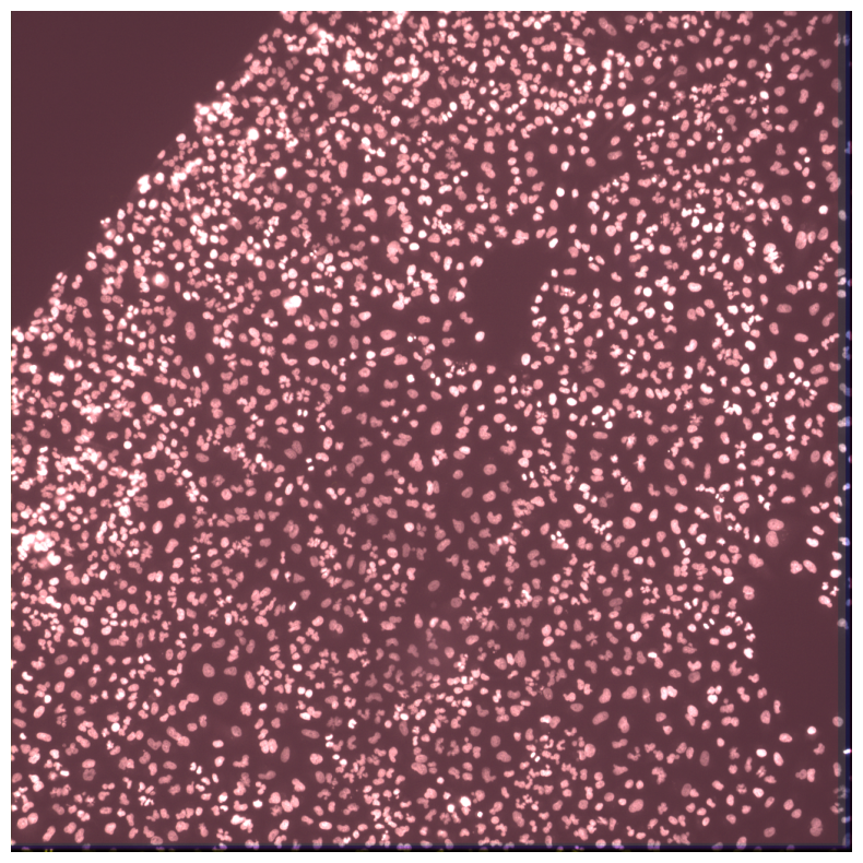
We can check how good the alignment is by either plotting a phenotype composite with the ISS labels or we can merge the two images and visualize the composite:

imcomposite(pheno_aligned, labels=nuclei, labels_contour=cells, figsize=(10, 10));

import xarray as xr

combined = xr.concat(
    [iss_image, pheno_aligned.expand_dims(["t"])], dim="c", join="outer"
)
imcomposite(combined.isel(c=dapi_channel), dim="t", figsize=(10, 10));

Compute Features

To compute the features you need to pass one of the features you want with the parameters for said features. In this example we will get the area, eccentricity and the correlation between DAPI (channel index 0) and NF-κB (channel index 1):

from scallops.features.find_objects import find_objects
from scallops.features.generate import label_features

objects_df = find_objects(cells)

phenotype_results = label_features(
    objects_df=objects_df,
    intensity_image=pheno_aligned.transpose(
        *("y", "x", "c")
    ).data,  # data needs to be transposed so that channel is last
    label_image=cells,  # You can pass any segmentation label
    features=["intensity_*", "size-shape"],
)

df_phenotype = objects_df.join(phenotype_results)
df_phenotype

measureobjectsizeshape.py (637): divide by zero encountered in divide
zernike.py (181): invalid value encountered in divide
zernike.py (184): invalid value encountered in divide

	AreaShape_BoundingBoxMinimum_Y	AreaShape_BoundingBoxMaximum_Y	AreaShape_BoundingBoxMinimum_X	AreaShape_BoundingBoxMaximum_X	AreaShape_Center_Y	AreaShape_Center_X	AreaShape_Area	AreaShape_BoundingBoxArea	AreaShape_ConvexArea	AreaShape_EquivalentDiameter	...	Intensity_IntegratedIntensityEdge_Channel0	Intensity_MeanIntensityEdge_Channel0	Intensity_StdIntensityEdge_Channel0	Intensity_MinIntensityEdge_Channel0	Intensity_MaxIntensityEdge_Channel0	Intensity_IntegratedIntensityEdge_Channel1	Intensity_MeanIntensityEdge_Channel1	Intensity_StdIntensityEdge_Channel1	Intensity_MinIntensityEdge_Channel1	Intensity_MaxIntensityEdge_Channel1
1	117	136	698	718	125.938525	708.340164	244.0	380.0	261.0	17.625846	...	0.515236	0.010103	0.003856	0.007797	0.026612	1.439216	0.028220	0.007859	0.019028	0.053559
2	418	440	355	378	427.787645	367.528958	259.0	506.0	352.0	18.159544	...	0.871229	0.009470	0.002003	0.007767	0.017273	2.553872	0.027759	0.003378	0.021912	0.036515
3	264	280	491	510	271.485000	500.485000	200.0	304.0	223.0	15.957691	...	0.490776	0.009438	0.001078	0.008225	0.012848	1.407126	0.027060	0.003307	0.020035	0.034806
4	208	228	663	676	217.015000	668.940000	200.0	260.0	221.0	15.957691	...	0.606455	0.011891	0.004497	0.007965	0.027039	1.345937	0.026391	0.003446	0.019196	0.035111
5	509	534	896	916	521.124113	906.379433	282.0	500.0	322.0	18.948708	...	0.674846	0.009780	0.002776	0.007721	0.021027	1.410269	0.020439	0.003635	0.013596	0.031800
...	...	...	...	...	...	...	...	...	...	...	...	...	...	...	...	...	...	...	...	...	...
2963	42	51	534	544	45.354167	539.437500	48.0	90.0	59.0	7.817640	...	0.257374	0.010295	0.002209	0.008026	0.016495	0.550072	0.022003	0.003705	0.016495	0.031434
2964	816	823	627	642	819.115942	634.565217	69.0	105.0	76.0	9.373021	...	0.358755	0.011958	0.003057	0.008164	0.017624	0.744167	0.024806	0.005798	0.014466	0.035080
2965	798	813	410	427	805.957265	418.205128	117.0	255.0	189.0	12.205287	...	0.674815	0.011063	0.004951	0.007691	0.025071	1.199924	0.019671	0.004311	0.014527	0.032441
2967	259	270	175	185	263.964286	180.571429	56.0	110.0	75.0	8.444016	...	0.391089	0.013036	0.003799	0.008179	0.020432	0.852430	0.028414	0.004930	0.018250	0.038239
2968	487	499	918	928	492.149254	922.970149	67.0	120.0	81.0	9.236182	...	0.390738	0.013025	0.005218	0.008042	0.026551	0.798428	0.026614	0.006177	0.019364	0.039643

2896 rows × 148 columns

import pandas as pd

from scallops.reads import merge_sbs_phenotype

merged_df = merge_sbs_phenotype(
    df_labels=df_cells,
    df_phenotype=df_phenotype,
    df_barcode=pd.read_csv(barcodes_path),
    sbs_cycles=iss_image.coords["t"].values,
)
merged_df

	mismatch	barcode_Q_mean	barcode_Q_min	barcode_peak	barcode_count	barcode_0	barcode_Q_mean_0	barcode_Q_min_0	barcode_peak_0	barcode_count_0	...	Intensity_MinIntensityEdge_Channel1	Intensity_MaxIntensityEdge_Channel1	barcode	sgRNA	gene_symbol	duplicate_prefix	barcode_1_barcode_1	sgRNA_1	gene_symbol_1	duplicate_prefix_1
1	False	360.0	360.0	3272.963489	6.0	AAATGATCT	360.0	360.0	3272.963489	6.0	...	0.019028	0.053559	AAATGGATCTATGTTCACAA	AAATGGATCTATGTTCACAA	FBXO32	False	NaN	NaN	NaN	NaN
2	True	180.0	180.0	1098.411341	3.0	AGGATTTAG	180.0	180.0	1098.411341	3.0	...	0.021912	0.036515	NaN	NaN	NaN	NaN	NaN	NaN	NaN	NaN
3	False	60.0	60.0	268.992267	1.0	GCTGTAGAC	60.0	60.0	268.992267	1.0	...	0.020035	0.034806	GCTGTGAGACCCAGCACCTG	GCTGTGAGACCCAGCACCTG	DHX58	False	NaN	NaN	NaN	NaN
4	False	300.0	300.0	1994.343939	5.0	GCTCTGCAG	300.0	300.0	1994.343939	5.0	...	0.019196	0.035111	GCTCTTGCAGGAATTTCCAG	GCTCTTGCAGGAATTTCCAG	USP17L2	False	NaN	NaN	NaN	NaN
5	False	300.0	300.0	2196.703452	5.0	ACTCAAAAC	300.0	300.0	2196.703452	5.0	...	0.013596	0.031800	ACTCACAAACAACATTGCTG	ACTCACAAACAACATTGCTG	IL6R	False	NaN	NaN	NaN	NaN
...	...	...	...	...	...	...	...	...	...	...	...	...	...	...	...	...	...	...	...	...	...
2963	NaN	NaN	NaN	NaN	NaN	NaN	NaN	NaN	NaN	NaN	...	0.016495	0.031434	NaN	NaN	NaN	NaN	NaN	NaN	NaN	NaN
2964	NaN	NaN	NaN	NaN	NaN	NaN	NaN	NaN	NaN	NaN	...	0.014466	0.035080	NaN	NaN	NaN	NaN	NaN	NaN	NaN	NaN
2965	False	180.0	180.0	1285.524961	3.0	CTCACTGCA	180.0	180.0	1285.524961	3.0	...	0.014527	0.032441	CTCACCTGCAATTAGGTGGA	CTCACCTGCAATTAGGTGGA	UBE2E1	False	NaN	NaN	NaN	NaN
2967	NaN	NaN	NaN	NaN	NaN	NaN	NaN	NaN	NaN	NaN	...	0.018250	0.038239	NaN	NaN	NaN	NaN	NaN	NaN	NaN	NaN
2968	False	60.0	60.0	64.093509	1.0	GCACGGTGG	60.0	60.0	64.093509	1.0	...	0.019364	0.039643	GCACGTGTGGCAGATCACGT	GCACGTGTGGCAGATCACGT	SPSB1	False	NaN	NaN	NaN	NaN

2896 rows × 173 columns

Post-processing results

After getting all the features and barcode results, we still need to process the data so it is clean and trustworthy.

Keep cells in which top barcode accounts for > 50% of aligned reads

The so-called 50% rule allows you to have more trust in your data. When you have multiple barcodes in a cell, you’d like that the top barcode represents more than 50% of all barcodes in the cell, such that you are sure the main effect in that cell is due to the intended guide. This filtering can easily be done in pandas:

filtered_merged_df = merged_df.query("barcode_count_0/barcode_count>0.5")
f"Kept {len(filtered_merged_df):,} / {len(merged_df):,} cells"

'Kept 2,146 / 2,896 cells'

Now lets visualize some important stats that allows you to gauge the reliability of the data.

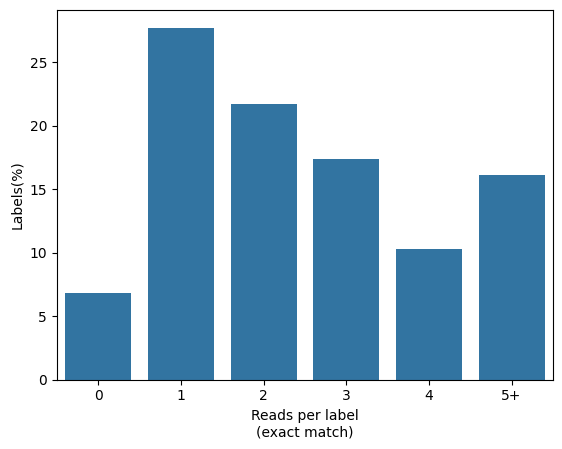
Percent of cells that contain barcode reads

We might want to know how many exact matches are respresented in cells. We can do this by using in_situ_barcode_hist_plot on the df_reads dataframe we computed earlier:

import matplotlib.pyplot as plt

from scallops.visualize.histogram import in_situ_barcode_hist_plot

in_situ_barcode_hist_plot(df_reads);

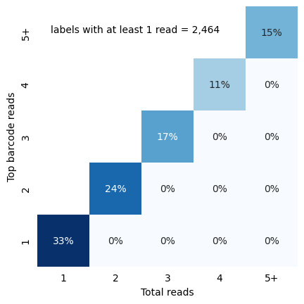
Cellular read distribution categorized by read identity

To visualize how the top barcode reads match the total number of reads, we can use the in_situ_identity_matrix_plot in the df_cells dataframe computed earlier:

from scallops.visualize.heatmap import in_situ_identity_matrix_plot

in_situ_identity_matrix_plot(df_cells.rename(columns={"barcode_0": "barcode"}));

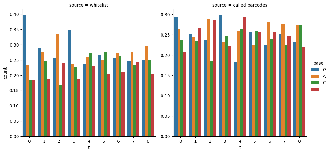
Whitelist and Called Barcodes Distribution

Once you have the called reads, you might want to compare them with your white list, especially in composition. We can use pandas and seaborn to that end:

import seaborn as sns

from scallops.reads import base_counts

barcode_counts_df = base_counts(
    df_barcode, normalize=True
)  # compute counts per base per cycle
barcode_counts_df["source"] = "whitelist"
called_barcode_counts_df = base_counts(df_reads, normalize=True)
called_barcode_counts_df["source"] = "called barcodes"
combined_counts = pd.concat((barcode_counts_df, called_barcode_counts_df))
sns.catplot(
    combined_counts,
    x="t",
    y="count",
    col="source",
    hue="base",
    kind="bar",
    sharey=False,
);

Fraction of neighbors with same target

You might also be wondering what is the proportion of neighbors have the same guide. This might be interesting to see the potential biases in guide uptake, and to see how uniform the experiment is. We can achieve this with scipy’s KDTree to find nearest neighbors based on coordinates of the filtered dataframe:

from scipy.spatial import KDTree

kdt = KDTree(
    filtered_merged_df[["AreaShape_Center_Y", "AreaShape_Center_X"]].values
)  # Create a K dimensional tree
neighbors = kdt.query_ball_tree(
    kdt, r=40
)  # Find all pairs of points between self and other whose distance is at most r.
neighbors_df = filtered_merged_df[["gene_symbol"]].copy()
fraction_same_gene = []
number_of_neighbors = []

for i in range(len(neighbors)):
    indices = neighbors[i]
    n = len(indices) - 1
    target_gene = neighbors_df["gene_symbol"].values[i]
    n_same = (neighbors_df["gene_symbol"].values[indices] == target_gene).sum() - 1
    fraction_same_gene.append(n_same / n if n > 0 else 0)
    number_of_neighbors.append(n)
neighbors_df["number_of_neighbors"] = number_of_neighbors
neighbors_df["fraction_same_gene"] = fraction_same_gene
neighbors_df = neighbors_df.sort_values("fraction_same_gene", ascending=False)
neighbors_df

	gene_symbol	number_of_neighbors	fraction_same_gene
2631	non-targeting	8	0.875000
1777	non-targeting	7	0.857143
1196	non-targeting	6	0.833333
1645	non-targeting	11	0.727273
1941	non-targeting	10	0.700000
...	...	...	...
2301	NaN	3	-0.333333
359	NaN	2	-0.500000
2878	NaN	2	-0.500000
867	NaN	2	-0.500000
2826	NaN	1	-1.000000

2146 rows × 3 columns